Does Predictor Order Affect the Results of Linear Regression?

Jakob Mar 2, 2021 R regression

In the last few weeks I encountered the following question in two separate discussions with friends and colleagues: When doing linear regression in R, will your coefficients vary if you change the order of the predictors in your data?

My intuitive answer to this was a clear “No”. Mostly because the practical implications of the alternative would be too severe. It would make linear regression unusable in many research settings in which you rely on the fitted coefficients to understand the relationship between the predictors and the independent variable. After all, what would be the correct, “canonical” order of inputs that you should use to estimate these effects?

The problem might be less relevant in other settings where you are more focused on building models with high predictive performance, like it is the case in many business applications. In these scenarios you are likely to be using more powerful, black box models such as XGBoost or random forest models to begin with. However, even then it is common practice to use a regression model as a baseline to better understand your data and benchmark your production models against.

So the issue seemed very relevant to me but I realised I did not have many arguments handy to support my intuitive answer. Therefore I decided to spend some time to explore the issue further and in the process refresh some of the numerical theory behind how the linear regression problem is solved on a computer.

Turns out that during the course of my investigation which I want to summarise in this blog post my simple “No” has become more of an “It depends…”

Note that I will only be looking at R’s standard linear regression function as implemented in the lm function from the stats package.

A First Look at the Problem

First of all, let’s try to get some more clarity about the exact question that we will be trying to answer here. Let’s say we are fitting two linear regression models on the good old mtcars dataset:

> m1 <-
+   lm(formula  = mpg ~ cyl + disp + hp + drat + wt + qsec + gear, data = mtcars)
> m2 <-
+   lm(formula  = mpg ~ qsec + hp + gear + cyl  + drat + wt + disp, data = mtcars)

These two models contain the same predictors, just in a different order. Now if we compare the fitted coefficients of both models, can we expect them to be the same?

So let’s put the coefficients of both models side by side and calculate their relative error:

##           key    coeff_m1    coeff_m2    rel_error
## 1 (Intercept) 18.58647751 18.58647751 1.338016e-15
## 2         cyl -0.50123400 -0.50123400 5.094453e-15
## 3        disp  0.01662624  0.01662624 1.043365e-15
## 4          hp -0.02424687 -0.02424687 1.430884e-16
## 5        drat  1.00091587  1.00091587 1.331049e-15
## 6          wt -4.33688975 -4.33688975 4.095923e-16
## 7        qsec  0.60667859  0.60667859 1.830002e-16
## 8        gear  1.04427289  1.04427289 6.378925e-16

So while the way the values are displayed suggests that they might be identical, we can see from the column rel_error that they are actually not exactly the same.

To make sure that this fluctuation is actually a result of the predictor permutation and not a result of some potential non-determinism within the lm function, let’s see what happens when we fit the exact same model twice:

> all(coefficients(lm(formula  = mpg ~ cyl + disp + hp + drat + wt + qsec + gear, data = mtcars)) ==
+       coefficients(lm(formula  = mpg ~ cyl + disp + hp + drat + wt + qsec + gear, data = mtcars)))
## [1] TRUE

It is reassuring to see that in this case the coefficients are exactly the same.

So here we have a first interesting finding: We can expect at least slight fluctuations in the coefficients when we play around with the order of the predictor variables.

Later on we will get a better idea where these small fluctuations come from when we look at how R solves the linear regression problem. However, at least in our example above, fluctuations on an order of \(\approx 10^{-16}\) will probably have no practical relevance. They also happen to be on the same order of magnitude as the machine precision for variables of type double.

Simulation Study

So after our little experiment with the mtcars dataset, can we consider our question answered? Not quite, as running two models on one single dataset can hardly be sufficient to answer such a general question.

For getting a more solid answer we will need to take a look at the theory of linear regression which we will do in a minute. But first let’s take an intermediate step and scale our little mtcars experiment to a larger amount of datasets. This will allow us to see if there are other, more severe cases of fluctuating coefficients and will also serve as a nice transition into the more theoretical parts of this post.

Getting Datasets from OpenML

To do this simulation study we obtained a number of datasets from the great OpenML dataset repository using their provided R package. Overall 207 datasets with between 25 and 1000 observations and between 3 and 59 predictors were obtained this way. This is obviously not a big sample of datasets to base general statements on. However, it should provide us with enough educational examples to get a better understanding and intuition of the kinds of issues you may encounter when fitting linear models “in the wild”.

The details and results from the study can be reviewed and replicated from the R Notebook here.

For each of the processed datasets we generated a number of predictor permutations and fitted a model for each of them using the same target variable each time. Overall we ended up with 3.764 fitted models with an average of 19.5 fitted coefficients each.

Quantifying the Coefficient Fluctuations

As we have already learned from our mtcars example above we can not expect the coefficients across different fits to be exactly the same. So we need to come up with a meaningful way to detect fluctuations that we would consider problematic.

For this we will use the coefficient of variation (CV) which is equal to the standard deviation normalised by the mean. It is therefore a measure of spread/variation of a set of observations but unlike the standard deviation it is expressed on a unit-less scale relative to the mean. This will allow us to compare the CVs of the different coefficients.

For every predictor in each dataset we calculated the CV across all the fit coefficients from the different models (i.e. predictor permutations). To identify extreme cases of fluctuations we flagged those predictors for which a CV of more than \(10^{-10}\) was measured. This limit has been chosen somewhat arbitrarily but should represent a quite conservative approach as it limits the maximum deviation for any given coefficient to \(\sqrt{N-1} * 10^{-10}\). Here \(N\) is the number of fits for that coefficient which in our case is between 2 and 20 depending on the dataset.

Simulation Results

In our simulation around 14.3 % of the coefficients showed a CV value above the chosen threshold of \(10^{-10}\), involving around 7.7 % of the datasets. The plot below also shows the overall distribution of the CV in a histogram on a log 10 scale.

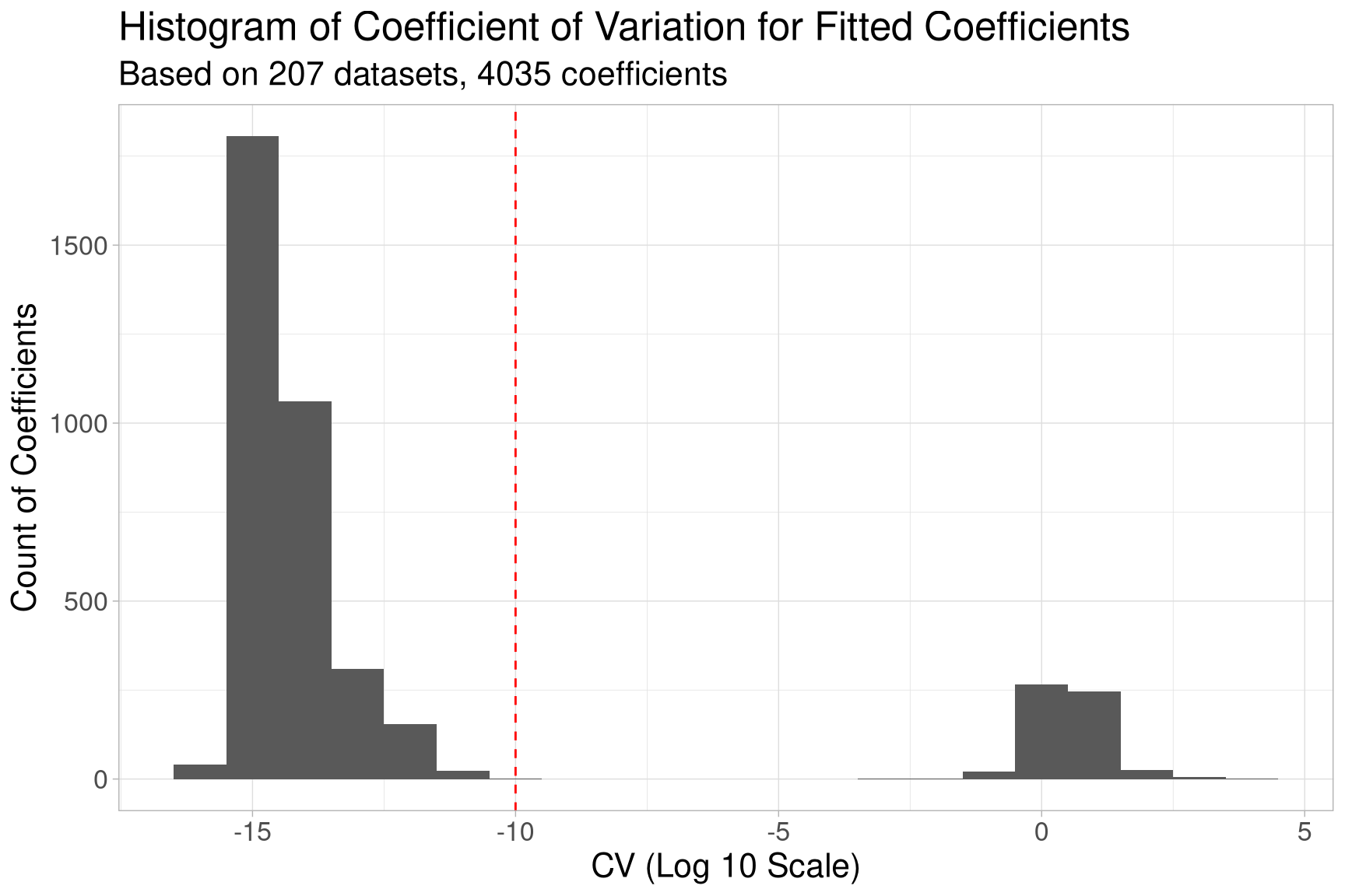
From the plot we can see that some of the coefficients fluctuate on a magnitude of up to \(10^3\), way above our defined threshold of \(10^{-10}\) (dashed red line). Unlike the fluctuations on the mtcars dataset these kinds of fluctuations can certainly not be ignored in practice.

Analysis

So let’s try to do some troubleshooting to find out how these fluctuations come about. First, let’s take a closer look at the datasets in which the problematic coefficients occur:

## # A tibble: 16 x 7
##    dataset_id  max_cv high_cv perc_coefficients_missi… dep_var      n_obs n_cols
##         <int>   <dbl> <lgl>                      <dbl> <chr>        <int>  <int>
##  1        195    2.64 TRUE                      0.0476 price          159     21
##  2        421 5321.   TRUE                      0.426  oz54            31     54
##  3        482   11.5  TRUE                      0.0217 events         559     46
##  4        487  410.   TRUE                      0.268  response_1      30     41
##  5        513    3.91 TRUE                      0.0217 events         559     46
##  6        518    1.02 TRUE                      0.222  Violence_ti…    74      9
##  7        521 1284.   TRUE                      0.118  Team_1_wins    120     34
##  8        527   11.3  TRUE                      0      Gore00          67     15
##  9        530    1.17 TRUE                      0.0833 GDP             66     12
## 10        533   35.0  TRUE                      0.0217 events         559     46
## 11        536   24.1  TRUE                      0.0217 events         559     46
## 12        543 2462.   TRUE                      0.111  LSTAT          506    117
## 13        551   30.5  TRUE                      0.188  Accidents      108     16
## 14       1051   70.4  TRUE                      0.238  ACT_EFFORT      60     42
## 15       1076  194.   TRUE                      0.383  act_effort      93    107
## 16       1091   49.8  TRUE                      0      NOx             59     16

One thing that stands out is that for almost all of the problematic datasets there seem to be coefficients that could not be fit (see column perc_coefficients_missing). This suggests that the lm function ran into some major problems while trying to fit some of the models on these datasets.

Underdetermined Problems

To understand how that happens let’s start by looking at a subset of the problematic cases: some of the datasets (dataset_ids 421, 487, 1076) contain more predictors than there are observations in the dataset (n_pred > n_obs). For linear regression this poses a problem as it means that we are trying to estimate more parameters than we have data for (i.e. the problem is underdetermined).

It is easy to understand the issue when thinking about a scenario in which we have only one predictor \(x\) and a target variable \(y\). Let’s say we try to fit regression model including an intercept (the offset from the y axis) and a slope for \(x\):

\[y = a + b*x\]

Further, let’s assume we only have one observation \((x,y) = (1,1)\) in our data to estimate the two coefficients \(a\) and \(b\) (n_pred > n_obs). It is easy to see that there are infinitely many pairs \(a\) and \(b\) that will fit our data, some of which are shown below:

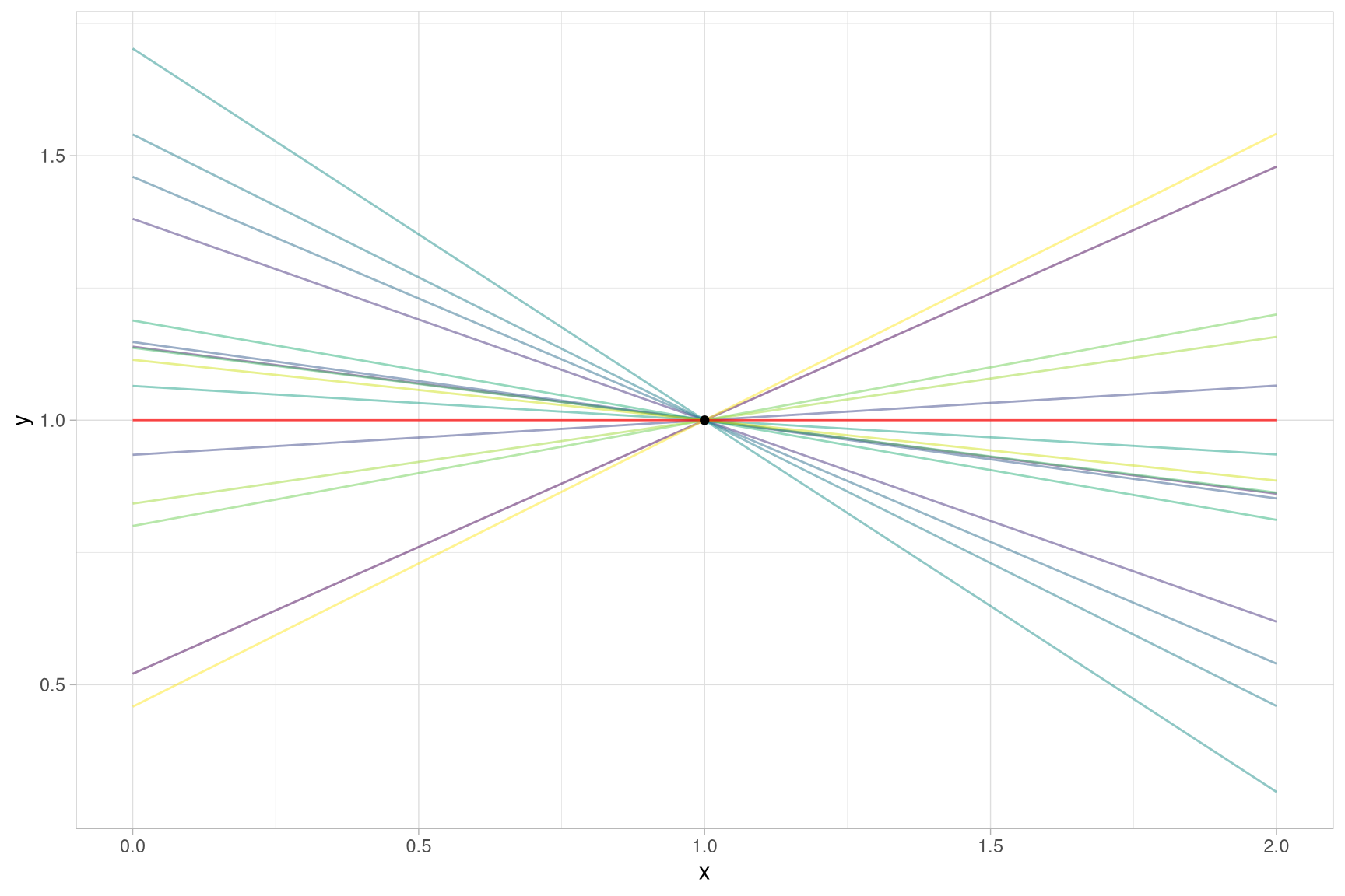
So when you are asking R to fit a linear regression in this scenario you are giving it somewhat of an impossible task. However, it will not throw an error (at least not when using the default settings). It will produce a solution, in our particular example the flat red line in the plot above:

> lm(y ~ ., data = tibble(x = 1, y = 1))
## 
## Call:
## lm(formula = y ~ ., data = tibble(x = 1, y = 1))
## 
## Coefficients:
## (Intercept)            x  
##           1           NA

So in the case of n_pred > n_obs we have an explanation for how the missing coefficients occur: R is “running out of data” for the surplus coefficients and will assign NA to them.

The running out of data part in the sentence above is a bit of a simplification. However, the estimation of coefficients seems to actually happen sequentially. At least that is the impression we get from a slightly more complicated example:

> example_2predictors <-
+   tibble(x1 = c(1, 2),
+          x2 = c(-1, 1)) %>%
+   mutate(y = x1 + x2)
> 
> lm(y ~ x1 + x2, data = example_2predictors)
## 
## Call:
## lm(formula = y ~ x1 + x2, data = example_2predictors)
## 
## Coefficients:
## (Intercept)           x1           x2  
##          -3            3           NA
> lm(y ~ x2 + x1, data = example_2predictors)
## 
## Call:
## lm(formula = y ~ x2 + x1, data = example_2predictors)
## 
## Coefficients:
## (Intercept)           x2           x1  
##         1.5          1.5           NA

We can see that at least in this example lm seems to prioritise the estimation of the coefficients in the order that we supply it to the model formula and assigns NA to the second predictor.

What is even better, the example also provides a case of fluctuating coefficients: The intercept in the first model is -3 and becomes 1.5 in the second one. And this intuitively makes sense as well. When we try to fit the model with too little data to estimate all the predictors what lm ends up doing is fitting a “reduced” model with fewer predictors. This limited set of predictors will explain the data in a different way and therefore result in different coefficients.

The Least Squares Problem

So now we have a pretty good understanding where the fluctuating coefficients originate from in the case of underdetermined problems as the ones above. The remaining datasets on the list above are not underdetermined but upon closer inspection we can see that they are suffering from the same underlying issue.

For this it is necessary to understand the theoretical foundation of how linear regression problems are solved numerically, the least squares method. A good and concise derivation of it can be found in these lecture notes.

The least squares formulation for linear regression turns out to be as follows:

\[X^tX\beta = X^tY\] In the equation above \(Y\) is the target variable we want to fit our data to and \(\beta\) is the vector holding the coefficients we want to estimate. \(X\) is the design matrix representing our data. Each of its \(n\) rows corresponds to one observation and each of its \(p\) columns to one predictor.

Now in order for us to solve the least squares problem we need the matrix \(X^tX\) to be invertible. If that is the case we can simply multiply both sides of the equation above by \((X^tX)^-1\) and have a solution for our coefficients \(\beta\).

However, for \(X^tX\) to be invertible it needs to have full rank. The rank is a fundamental property of a matrix which has many different interpretations and definitions. For our purposes it is only important to know that \(X^tX\) would have full rank if its rank would be equal to the number of its columns \(p\) (which in our case is the same as the number of predictors). By one of the properties of the rank, the rank of \(X^tX\) can at most be the minimum of \(n\) and \(p\).

Now we can see why we ran into problems when we tried to fit a linear regression model for the datasets that had less observations (\(n\)) than predictors (\(p\)): The matrix \(X^tX\) had rank \(< p\) (i.e. not full rank) and was therefore not invertible.

As a consequence the underlying least squares problem for these cases was not solvable (at least not in a proper way as we will see in a bit).

Multicollinearity

With our understanding of the underdetermined problems and the issues they cause in the least squares formulation we now have all the necessary tools to explain all the other cases of fluctuating coefficients. As we have pointed out the remaining cases are not underdetermined (\(p\) > \(n\)), instead they suffer from a slightly more subtle issue called multicollinearity.

Multicollinearity arises when some of the columns in your data can be represented as a linear combination of a subset of the other columns.

For example, the columns of the following dataset have multicollinearity:

## # A tibble: 5 x 4
##       y    x1    x2    x3
##   <dbl> <dbl> <dbl> <dbl>
## 1     1     1    -1     0
## 2     1     2     1     3
## 3     1     3    -1     2
## 4     0     4     1     5
## 5     0     5    -1     4

If we know two of the three predictor columns we can always calculate the third (e.g. x1 = x2 + x3). One of the columns is simply representing the same data as the other two in a redundant fashion. We could remove either one of them and still retain the same information in the data.

It might not be clear at first sight why having additional columns that represent the same data in a redundant way should pose problems but it becomes obvious when we analyse it with the same tools that we used above.

One of the definitions for the rank of a matrix is the number of linearly independent columns. But as we have just seen in a dataset with multicollinearity some of the columns will be linear combinations of other columns. Therefore if our matrix \(X\) has multicollinearity in its columns its rank will be less than the number of its columns \(p\). And since \(rank(X^tX) = rank(X) < p\) this means that \(X^tX\) is not invertible.

Therefore we can trace the remaining cases of fluctuating coefficients back to the \(n < p\) case and explain them in the same way!

Multicollinearity can be a bit difficult to detect sometimes but it can be found in all of the remaining datasets in which we have detected the coefficient fluctuations (see the accompanying R notebook document). In the case of datasets 527 and 1091 we have a special case where we have collinearity between the predictors and the target variable which can also explain why there are no missing coefficients in these cases.

Why lm still returns results: QR Decomposition

So we have been able to explain all the cases of coefficient fluctuations by violations of basic assumptions of linear regression that every undergraduate textbook should warn you about:

make sure you have at least as many observations as predictors you want to fit
make sure your data has no multicollinearity in it

However when we tried to fit a linear regression R was able to provide us with results (albeit some of the coefficients were missing) without any error or even warning.

How can it come to any solution if the inverse of \(X^tX\) in the matrix formulation above does not exist?

To understand this it is necessary to dive a bit deeper into the internal workings of the lm function in R. I highly recommend doing that as it will teach you a lot about how R works internally and how it interfaces with other languages (the actual code for doing the matrix inversion is using Fortran code from the 1970s). This blog post offers a great guide to follow along if you are interested in those implementation details.

The bottom line for us here is that to solve the linear regression problem R will try to decompose our design matrix \(X\) into the product of two matrices \(Q\) and \(R\). With this factorization it becomes quite straightforward to solve the overall matrix equation for our coefficient vector \(\beta\).

Now without going into too much detail here, we can say that the QR decomposition can be executed even when \(X\) is not invertible as the computations are essentially done for each coefficient sequentially.

So the QR and will produce meaningful values for the first few coefficients up until the algorithm will abort the calculation and return NA for the remaining coefficients. This is exactly the behaviour we have seen in our little example datasets above and in our simulation study.

I was a bit surprised to see that R will just silently process the data even if it encounters these kinds of problems with the QR decomposition (I certainly remembered the behaviour differently). The lm function actually provides a way to change this behaviour by setting the singular.ok to FALSE. In this case lm will error out when it runs into a matrix with non-full rank and not return any results. The default for this parameter however is set to TRUE resulting in the behaviour we have witnessed in our analysis. Interestingly the help text of the lm function mentions that this parameter’s default was FALSE in R’s predecessor S.

The output of lm provides some information about the QR fit, most importantly the rank of the matrix it encountered, which can be extracted from the output. So let’s append this information to all our datasets in which we found fluctuations in the coefficients:

## # A tibble: 16 x 8
##    dataset_id high_cv perc_coefficient… dep_var n_obs n_cols rank_qr singular_qr
##         <int> <lgl>               <dbl> <chr>   <int>  <int>   <int> <lgl>      
##  1        195 TRUE               0.0476 price     159     21      20 TRUE       
##  2        421 TRUE               0.426  oz54       31     54      31 TRUE       
##  3        482 TRUE               0.0217 events    559     46      45 TRUE       
##  4        487 TRUE               0.268  respon…    30     41      30 TRUE       
##  5        513 TRUE               0.0217 events    559     46      45 TRUE       
##  6        518 TRUE               0.222  Violen…    74      9       7 TRUE       
##  7        521 TRUE               0.118  Team_1…   120     34      30 TRUE       
##  8        527 TRUE               0      Gore00     67     15      15 FALSE      
##  9        530 TRUE               0.0833 GDP        66     12      11 TRUE       
## 10        533 TRUE               0.0217 events    559     46      45 TRUE       
## 11        536 TRUE               0.0217 events    559     46      45 TRUE       
## 12        543 TRUE               0.111  LSTAT     506    117     104 TRUE       
## 13        551 TRUE               0.188  Accide…   108     16      13 TRUE       
## 14       1051 TRUE               0.238  ACT_EF…    60     42      32 TRUE       
## 15       1076 TRUE               0.383  act_ef…    93    107      66 TRUE       
## 16       1091 TRUE               0      NOx        59     16      16 FALSE

We can see that almost all of the datasets with coefficient fluctuations have encountered a singular QR decomposition. The only two exceptions we have found (datasets 527 and 1091) have another defect are the ones we mentioned above where there is collinearity between the target variable and the predictors. The issue with those datasets has therefore a slightly different nature (see details in the R notebook) but they definitely represent ill-posed linear regression problems.

As a side note: The QR decomposition is calculated only approximated using numerical algorithms (in the case of R Householder reflections are used). The approximative nature of the calculations is likely to be the reason for the minimal coefficient fluctuations we have seen in the mtcars example and our simulation study.

Pivoting in Fortran

One final thing I came across while trying to make sense of the Fortran code which does the actual QR decomposition is that it is applying a pivoting strategy to improve the numerical stability of the problem. You can find the code and some documentation about the pivoting here.

The application of the pivoting strategy implies that in certain cases the Fortran function will try to improve the numerical stability of the QR decomposition by moving some of the columns to the end of the matrix.

This behaviour is relevant for our analysis here as it means there is some reordering of the columns going on which we do not have any control over in R.

This might influence our results as it might be the case that for those datasets in which we found no fluctuations it was simply because our prescribed column ordering was overwritten in the Fortran code and never had the chance to cause coefficient fluctuations.

Again the information whether pivoting was applied is returned in the output of the lm function so let’s append this information to our dataset summary and filter for all datasets on which pivoting was applied:

## # A tibble: 18 x 7
##    dataset_id   max_cv high_cv perc_coefficients_m… rank_qr singular_qr pivoting
##         <int>    <dbl> <lgl>                  <dbl>   <int> <lgl>       <lgl>   
##  1        195 2.64e+ 0 TRUE                  0.0476      20 TRUE        TRUE    
##  2        199 6.72e-15 FALSE                 0.143        6 TRUE        TRUE    
##  3        217 2.00e-14 FALSE                 0.0357      27 TRUE        TRUE    
##  4        421 5.32e+ 3 TRUE                  0.426       31 TRUE        TRUE    
##  5        482 1.15e+ 1 TRUE                  0.0217      45 TRUE        TRUE    
##  6        494 0.       FALSE                 0.333        2 TRUE        TRUE    
##  7        513 3.91e+ 0 TRUE                  0.0217      45 TRUE        TRUE    
##  8        518 1.02e+ 0 TRUE                  0.222        7 TRUE        TRUE    
##  9        521 1.28e+ 3 TRUE                  0.118       30 TRUE        TRUE    
## 10        530 1.17e+ 0 TRUE                  0.0833      11 TRUE        TRUE    
## 11        536 2.41e+ 1 TRUE                  0.0217      45 TRUE        TRUE    
## 12        543 2.46e+ 3 TRUE                  0.111      104 TRUE        TRUE    
## 13        546 1.94e-13 FALSE                 0.0769      24 TRUE        TRUE    
## 14        551 3.05e+ 1 TRUE                  0.188       13 TRUE        TRUE    
## 15        703 1.17e-11 FALSE                 0.104      302 TRUE        TRUE    
## 16       1051 7.04e+ 1 TRUE                  0.238       32 TRUE        TRUE    
## 17       1076 1.94e+ 2 TRUE                  0.383       66 TRUE        TRUE    
## 18       1245 8.26e-15 FALSE                 0.115       23 TRUE        TRUE

As we can see pivoting was only applied in datasets where we also encountered a singular QR decomposition which makes sense as putting a non-invertible matrix into the algorithm probably has poor numerical stability. Out of those datasets there are a total of 6 datasets where pivoting was applied but no coefficient fluctuations were detected. Whether the pivoting had an impact in preventing the fluctuations from happening or if it was another property of the dataset is hard to say.

Either way we can conclude that the pivoting has not interfered with the results of the vast majority of the datasets in which we did not see any fluctuations.

Conclusion

We started this post with a seemingly trivial question which in the end took us on quite a journey which involved a simulation study, revisiting the linear algebra behind the linear regression problem and taking a closer look at how the resulting matrix equations are solved numerically in R (or rather in Fortran).

All the cases of coefficient fluctuations we could detect in our investigation were caused by violations of basic assumptions of linear regression and not the permutations of the input variables per se.

Therefore our conclusion is that as long as you do your due diligence when fitting regression models you should not have to worry about the order of your predictors having any kind of impact on your estimated coefficients.