Comparing Restaurant Reviews in Stockholm and Berlin

Late last summer we spent a couple of weeks on vacation in beautiful Sweden. Back then the Corona pandemic had not yet hit the country quite as hard and it was still possible to go to restaurants without any restrictions. While looking online for nice restaurants to go to we noted some differences in the user reviews from what we were used to from Germany.
On the one hand we felt we encountered way less ratings that gave the full point score. This does not necessarily mean that restaurant quality is worse in Sweden than in Germany as there are many factors that make a direct comparison of these ratings difficult (as we’ll see below). However, this finding made me curious to investigate whether this difference can be substantiated in a larger dataset of reviews or whether it might be just a subjective impression we got from our small sample.
Another thing we noticed was an apparent difference in the wording of the review texts and how they relate to the point score. For example, let’s look at some actual reviews from Stockholm:
“Extremely tasty, fresh spicy burgers and fantastic sweet potato fries.”
“Very good food but the best thing is the staff, they are absolutely wonderful here!!”
“Stockholm’s best kebab I think. The pizzas are also super here.”
“Very good pasta, wonderful service !!! Very cozy place, everything is perfect👍”
While all of the review texts above seem to be overwhelmingly positive they were all associated with a point rating of less than five (the full score). From our personal experience with restaurant reviews from Germany (and Berlin specifically) we would have expected these review texts to indicate a five point rating.
Again, all of our observations were obviously subjective and we were only looking at a small, non-representative sample of restaurant reviews. Therefore I decided to find out whether our observations could actually be backed up by an analysis of a larger dataset of reviews.
To be precise, I would like to answer the following two questions:
- Is there a difference in the distribution of point ratings of restaurants when comparing Sweden and Germany?
- Is there a difference in the relationship between the wording of the review texts and the associated point rating?
I will answer these two questions over the course of two blog posts. This first post will describe how to obtain and process the review data. Once this is done answering the first question will be straightforward.
Answering the second question will be a bit more tricky, partly due to its somewhat vague formulation. It will require some Natural Language Processing (NLP) and modeling techniques and will be done in a dedicated follow-up post.
Getting the data
First of all, we will need to collect a sample of restaurant reviews from both countries that we can then analyse. For simplicity we will restrict our analysis to the two capital cities Berlin and Stockholm. As a data source we will query Google Maps through their public APIs.
Getting a Random Sample of Reviews
For our analysis it would be preferable to obtain a random sample of restaurant reviews from each of the cities as this will give us the most accurate estimation of the actual reality. The Google Maps API is not really designed to provide this kind of access so we will have to come up with a process that will at least approximate a random sample as close as possible. We will describe this process in this section.
The Place Details and Nearby Search APIs
The API endpoint that will provide the actual restaurant reviews is the
Place Details
endpoint. As one of its inputs it requires a place_id which uniquely identifies a
place (in our case a restaurant) within Google Maps. Given this identifier the
API will return some information about the restaurant, among them up to five user
reviews.
To obtain the place_ids of a number of restaurants in Berlin and Stockholm we
will use a second endpoint, the
Place Search. This endpoint provides the Nearby Search
functionality that accepts a set of latitude and longitude coordinates and will
return a list of up to 20 restaurants in proximity of these coordinates.
So to kick off our our process of sampling restaurant reviews all we need is a number of coordinates in Berlin and Stockholm respectively.
Sampling Coordinates within the Cities
Since we would like our final sample of reviews to be as random as possible it makes sense to randomly select coordinates in the two cities. Possibly the simplest way to do that would be to sample in the bounding box of each city which can be interpreted as a rectangular approximation of a city’s boundaries.
Using this approach we would get a sample of coordinates similar to the data we can see below (note that the zoom levels of the plots are different):
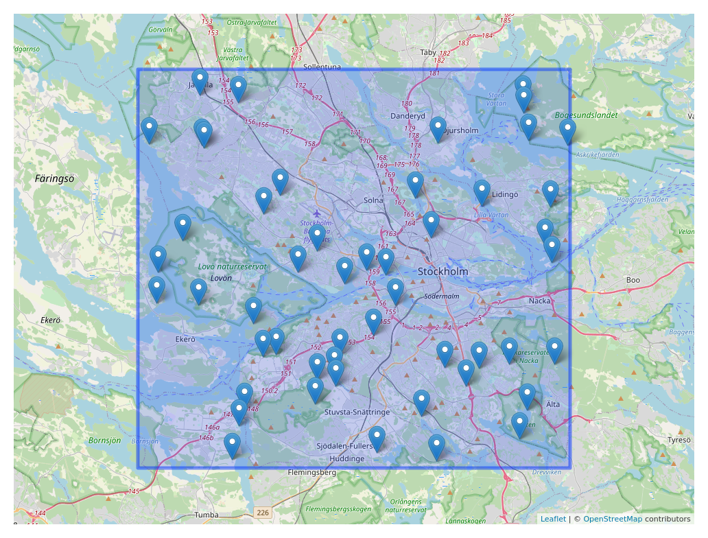

We can see that this approach seems to be quite inaccurate and inefficient as it produces many points outside the actual city limits.
Therefore we will turn to a more precise method using polynomial city boundaries
which can be obtained from the
Open Street Map project. Sampling coordinates
from this more complex geometric structure is not as straightforward as for the
rectangular bounding box but luckily it has already been implemented in the
spsample function from the R package sp.

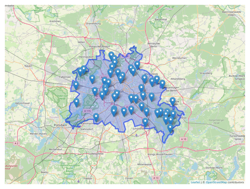
The results we get with this approach indeed seem to be preferable over the rectangular bounding box.
So now that we have a way to sample random locations within each of the cities we have defined the full process for obtaining restaurant reviews:
- Sample a number of coordinates for each city
- For each of the coordinates query the Nearby API for restaurants to obtain a
number of
place_ids - For each of the
place_ids query the Details API to get the restaurant reviews
Since this way of sampling may return the same review more than once we will have to deduplicate the results afterwards.
Language of Reviews
One more thing to note is that the Details API has a parameter which will control the language in which the reviews are returned. For our analysis it would intuitively make sense to set this parameter to English as it will make it easier to understand and process the data, especially for the second part of our investigation in which we will look at the review texts specifically.
However, while experimenting with different settings we found out that this parameter seems to do more than to simply return a one-to-one translation of the same reviews. In fact, in some cases it would yield completely different reviews.
So for our analysis we decided to set this parameter to the native language of the respective city. We did so in the hopes that we will obtain more reviews that were written by actual residents of the city this way. This should somewhat mitigate the influence of tourists on the ratings and allow us to get a clearer picture of the actual difference between the two cities.
Another added benefit of this approach is that it will force us to perform the translation ourselves which will also ensure that the review texts have gone through the same translation step. This additional step will be done through the Google Translation API.
Implementation
To actually query the Google Maps and Translation APIs we wrote simple one-liner functions, such as the one shown below for the Nearby API:
query_nearby_api <-
   function(x,y,api_key) {
      list(fromJSON(paste0("https://maps.googleapis.com/maps/api/place/nearbysearch/json?location=",y,",",x,"&rankby=distance&type=restaurant","&key=",api_key)))
   }
Now if we have our sampled coordinates in a dataframe where each row corresponds to
one set of coordinates we can query the API simply by wrapping the function above
in an mcmapply call:
results_nearby$nearby_response <-
   mcmapply(FUN = query_nearby_api,
            results_nearby$x,results_nearby$y,
            api_key,
            mc.cores = num_cores)
This has the added benefit of straightforward parallelisation though it should be noted that you may run into rate limits if you turn up the number of concurrent requests too much.
We applied a similar approach for all the APIs used in this analysis. If you are interested in the details you can find the full R implementation of the data collection process here.
Please note that if you want to replicate the results you will need to set up a Google Maps API key and running the script will incur costs depending on the amount of reviews you wish to query. Please check the the latest API pricing of Google Maps beforehand.
It should be mentioned that there are several R packages available which we could have used for querying the Google Maps APIs such as mapsapi or googleway. However, none of the packages we found offered access to all the APIs we needed to use (Nearby, Places Details, Translate) and since the APIs are pretty simple we decided to go with approach outlined above. This also gives us more control over other aspects such as the output format and the parallelisation.
Rating Distribution
Using the process described above we obtained a total of 32,376 restaurant reviews out of which 21,548 were from Berlin and 10,828 from Stockholm. As we can see our sample is not balanced even though we queried the same amount of coordinates for each city which is probably due to less restaurants or a lower restaurant density in Stockholm.
The review data comes out of our querying script in a handy dataframe format in which each row corresponds to one review:
## # A tibble: 32,376 x 9
##    city_name text_translated rating country_code country_language name  place_id
##    <chr>     <chr>            <int> <chr>        <chr>            <chr> <chr>
##  1 Berlin    "Today I got k…      4 de           de               Hacı… ChIJHZN…
##  2 Berlin    "I can only ag…      1 de           de               Suma… ChIJL3j…
##  3 Stockholm "Since Friday'…      1 se           sv               T.G.… ChIJt9T…
##  4 Berlin    "Super!!! Shor…      5 de           de               Curr… ChIJRQC…
##  5 Berlin    "Delicious, fr…      5 de           de               Brus… ChIJlx7…
##  6 Berlin    "Since there a…      4 de           de               Asia… ChIJf3D…
##  7 Berlin    "Quality for d…      5 de           de               Rist… ChIJIyF…
##  8 Stockholm "Thursdays are…      5 se           sv               Inte… ChIJo89…
##  9 Berlin    "Better than t…      3 de           de               Gril… ChIJX9r…
## 10 Berlin    "Sun, good Aug…      4 de           de               Zoll… ChIJiXM…
## # … with 32,366 more rows, and 2 more variables: place_rating <dbl>, text <chr>
With this data answering our first question about whether there is a difference in the point rating distributions of Stockholm and Berlin can easily be done by creating a simple visualisation of the two distributions:
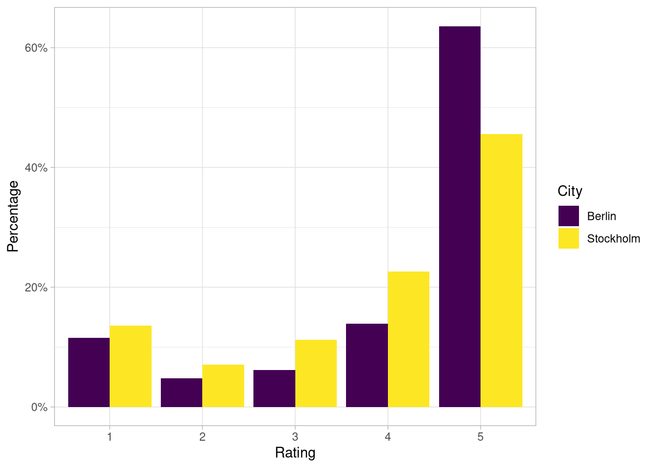
So it seems that there is actually quite a difference in the distributions of the two cities. In fact there are about 18 % more five point reviews in Berlin than in Stockholm and the difference seems to be spread out across all the remaining rating categories. The average rating in Berlin is 4.1 vs 3.8 in Stockholm.
The differences in the distribution are highly significant which can be confirmed by running a Chi Square test or (probably more appropriately) a Mann-Whitney U Test.
Comparability of Ratings from Berlin and Stockholm
So we have answered our first question whether the rating distribution for the two city differs.
But can we conclude from this that the restaurant quality in Berlin is higher than in Stockholm? At least from my personal experience this is not likely to be the case and there are also many theoretical arguments that could be made against this conclusion.
One pretty simple and obvious one can be made by looking a bit closer at the rating process. The point rating in Google Maps is a one-dimensional measure that aims to summarise the user’s impression of a location or service in one single number.
However, it is plausible to assume that in reality that a person’s opinion of a restaurant is formed by many different aspects such as the taste of the food, the atmosphere, value for money, quality of service etc.
For example, let’s assume the following simple model for the overall point rating a user will give to a restaurant:
\[s = w_{food} \cdot s_{food} + w_{atmosphere} \cdot s_{atmosphere} + w_{price} \cdot s_{price} + w_{service} \cdot s_{service}\]
Here the \(w\)s are weights that sum to one and indicate how much importance a user attributes to a certain aspect of the restaurant experience. The \(s\) variables hold sub scores (ranging from one to five) that a user would give to the aspect of the restaurant experience. So in our simple model the overall score a user gives to a restaurant is just a weighted sum of all those sub scores.
Let’s further assume that for different individuals the aspects above vary in importance for their overall satisfaction with their restaurant experience. This would translate into different sets of weights \(w\) for different users in the equation above, resulting in user-specific rating models:
\[s_{user1} = 0.5*s_{food} + 0.2*s_{atmosphere} + 0.2*s_{price} + 0.1*s_{service} \\ s_{user2} = 0.3*s_{food} + 0.2*s_{atmosphere} + 0.3*s_{price} + 0.2*s_{service}\]
Now what that means is that even if these two users agree in their assessment for each of the sub scores for a given restaurant, they might still come up with different overall scores for the same place. Accordingly the rating of the first user may have only limited relevance for the second user when choosing a restaurant (and vice versa).
The same argument holds on the city level: If the rating models of the people in Stockholm and Berlin differ too much from each other the ratings become incomparable.
And even if the rating models were to be the same in the sense that they share the same values for the weights \(w\) that still does not guarantee that the overall scores are compatible. For this we would still need the sub scores \(s\) to be identical for each user which may very well not be the case. For example, maybe people from Stockholm are (on average) more picky when it comes to the atmosphere of a restaurant and may assign a score of four for that aspect where a user from Berlin might assign a five point score.
The derivations above are of course only theoretical and hinge on many simplifying and unproven assumptions. Establishing how the rating process works in reality is probably not possible with the data we have available here.
However, the argument we are making above was only to discourage us from jumping to premature conclusions about the actual restaurant quality in the two cities when comparing their rating distribution. We have presented one possible scenario in which this comparison could lead to the wrong conclusion but are not claiming this is necessarily the case. In reality it might still very well be that Berlin simply has better restaurants than Stockholm! 😉
Entropy Considerations
So even though the rating distributions from the two cities may not tell us which city has the better restaurants, is there maybe something else we can learn from them?
In fact we could think about which of the two distributions provides a more realistic picture of the restaurant quality in the respective city which would have a direct impact on their usefulness for choosing a good restaurant.
As we have already discussed the Berlin distribution is heavily concentrated in the five point category (around 64 % of all ratings are in that category) whereas the Stockholm distribution is much more spread out among all categories.
We can think of the two distributions as more nuanced versions of two extreme cases: the uniform distribution (Stockholm) and a polarised one that is only concentrated in two categories (Berlin).
The plot below shows how these two distributions could look like:

The fact that the Berlin distribution is closer to the polarised distribution and the Stockholm distribution closer to the uniform can also be verified by calculating their respective entropies:
## # A tibble: 2 x 2
##   city_name entropy
##   <chr>       <dbl>
## 1 Berlin       1.13
## 2 Stockholm    1.40
Entropy is a measure from information theory and can be interpreted as a measure for how much information is encoded in a distribution.
Now how does this relate to the usefulness in picking a restaurant in the respective cities? This depends a bit on what we believe the actual landscape of restaurants in the two cities looks like.
If for example you believe that the vast majority of Berlin restaurants are top notch then such a heavily polarised distribution may actually provide you with an accurate picture of that reality.
Similarly, if you think that the Stockholm restaurant scene is closer to a pretty uniform mix of restaurants of all kinds of quality then the somewhat uniform shape of the rating distribution we have seen for Stockholm might be doing a good job.
On the other hand, if you doubt either of the two assessments above you could conclude that the respective distribution is not accurately reflecting reality and therefore not doing a good job at helping you to choose a nice restaurant.
A related side note from my personal experience: In Berlin I have been asked on several occasions by restaurant owners, doctors or Uber drivers to give them an online review in case I was happy with the service. However, they asked me to only leave a review if I was planning to give the full five point score as otherwise it would hurt their overall rating.
Having been made aware of these circumstances has actually changed my rating behaviour in general. I now tend to give the highest rating when I am at all satisfied in order to not hurt the restaurant’s or service provider’s overall standing. Therefore I am personally contributing to the polarised and potentially less informative rating distribution in Berlin. If this nudge effect is present in a sufficient amount of people it can partly explain the high polarisation in the distribution.
Conclusion
In this blog post we described how to obtain restaurant review data from the Google Maps APIs and compared the point rating distribution of Stockholm and Berlin.
Based on our sample of restaurant reviews we were able to verify our subjective impression that there are proportionally more five point ratings in Berlin than in Stockholm.
While we demonstrated that it will be difficult to draw any conclusions about which city has the better restaurants with this data, we could still discuss which distribution might be more informative to the user.
In the next blog post we will investigate whether there are discernible differences in the relationship between the review texts and the associated point rating between the two cities.