Sentiment Analysis for Restaurant Reviews in Stockholm and Berlin

In our previous blog post we posed two questions about restaurant reviews from Stockholm and Berlin. Using some actual restaurant review data from Google Maps we were able to find an answer to the first question about whether there is a difference in the point rating distribution between the two cities.
In this post we will focus on the second question which concerns the relationship between the review texts and the point score and how this relationship might differ between the two cities.
As a reminder, in Stockholm we encountered some review texts such as the ones below:
“Extremely tasty, fresh spicy burgers and fantastic sweet potato fries.”
“Very good food but the best thing is the staff, they are absolutely wonderful here!!”
“Very good pasta, wonderful service !!! Very cozy place, everything is perfect👍”
From our experience with restaurant reviews from Berlin we would have expected those reviews to be associated with a full five point score. However, all the reviews above had a rating of four or less.
This observation led us to formulate the following question:
Is there a difference in the relationship between the wording of the review texts and the associated point ratings between Stockholm and Berlin?
This question is pretty vague and can not really be answered using data analysis techniques. Therefore in this blog post we will concentrate on answering a more refined and specific version of this question:
Is there a difference in the sentiments in the restaurant review texts between Stockholm and Berlin?
If we can find a way to quantify the sentiment of a given text we can use this measure to compare the review texts from both cities. In particular this will allow us to check if there is a tendency for more positive wording in Stockholm reviews compared to the ones from Berlin. The existence of such a pattern would provide evidence to support our subjective observations.
Sentiment Analysis
To obtain such a measure we will use tools from the field of Sentiment Analysis which aims to quantify the sentiment that is expressed in a piece of text (single words, sentences or collections of sentences).
The typical output of these algorithms is a numerical value that gauges the strength of the sentiment of a given text. Examples for these sentiments can be the simple distinction into positive and negative sentiments or more refined emotional categories such as joy, anger or frustration.
For our analysis we will focus on classifying the review texts into the two opposing categories of negative and positive sentiments. The tools we will be using will produce a low score for a text which is estimated to have a negative sentiment and high scores for a text which is supposed to express a positive sentiment.
For example, in the context of restaurant reviews we would expect the first statement below to receive a high score while the second one should receive a low score:
“This is a great restaurant, very friendly staff and amazing food.”
“Do not go to this restaurant, the food tastes disgusting and the service is horrible!”
Sentiment analysis methods come in many different implementations and levels of complexity. In this blog post we will introduce and apply three different methods and compare their results.
For this we will use the same data as in our previous blog post but will now include the reviews texts that come with the point rating. The R and Python code to replicate the results from this analysis can be found here.
Lexicographical Approach
One very basic approach to generate a sentiment score from a piece of text is to assign a numeric value to each word (e.g. -1 to the word bad and +3 to the word amazing) and then simply aggregate all these individual scores.
An example for such a calculation is shown below:
\[\underbrace{\text{This }}_{0} \underbrace{\text{is }}_{0} \underbrace{\text{a }}_{0} \underbrace{\text{great }}_{+3} \underbrace{\text{restaurant}}_{0}, \underbrace{\text{very }}_{0} \underbrace{\text{friendly }}_{+2} \underbrace{\text{staff }}_{0} \underbrace{\text{and }}_{0} \underbrace{\text{amazing }}_{+4} \underbrace{\text{food}}_{0} .\] The overall sentiment score for this sentence would then be obtained by calculating the sum or the average of the individual scores.
Defining the sentiment scores for the individual words is not a trivial task but luckily there are a number of sentiment lexicons available that provide these kind of scores so we don’t have to create them ourselves. The Text Mining with R book describes how some of these lexicons can be accessed using their tidytext package.
For our analysis we will use the AFINN lexicon which was built on Twitter data and provides a score ranging from -5 (negative sentiments) to +5 (positive sentiments) for 2,477 words. Below is an example of those scores from the AFINN lexicon:
## # A tibble: 10 x 2
##    word        value
##    <chr>       <dbl>
##  1 stabs          -2
##  2 threaten       -2
##  3 debonair        2
##  4 disparaging    -2
##  5 jocular         2
##  6 fun             4
##  7 resolves        2
##  8 dirtiest       -2
##  9 goddamn        -3
## 10 joyous          3
One interesting thing to note is that the AFINN lexicon is skewed towards negative scores, around 64.5% of the entries in the lexicon have a negative score.
The authors of the Text Mining with R book also provide a process with which the sentiment scores can be calculated through simple dataframe transformations. We used this approach to calculate a score for each review as the average score of the words within it (assigning zero to words that were not contained in the dictionary).
Taking the average of these scores within each point rating category and breaking it down by city yields the following distribution:
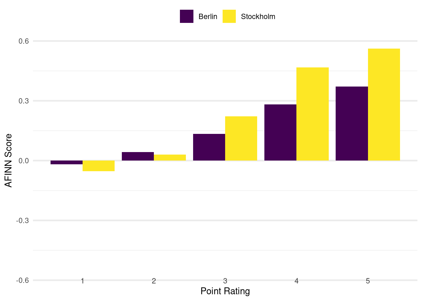
The overall pattern for the sentiment score distribution is the same for both cities: Higher point ratings are associated with higher sentiment scores. This finding makes intuitive sense and is a good face validity check of this method.
When we compare the scores between the two cities within each point rating group we can see that the Stockholm scores are more polarised in each category: They are lower for the two bottom categories (ratings of one and two points) and higher for the top two categories (four and five points) than the scores from Berlin.
Going back to our analysis question this finding seems to support our subjective observations: On average the review texts in the four and three point categories in Stockholm express more positive sentiments than the ones in Berlin. The average sentiment score in the four point category for reviews from Stockholm is even higher than the score for five point reviews in Berlin. It is therefore plausible that in Stockholm we are likely to come across four point reviews that we would assume to be five point reviews (based on our experience from Berlin).
Issues with the Lexicographical Approach
The lexicographical approach is very simple to understand and implement. However, its simplicity also results in some limitations. One obvious drawback is the handling of more complex sentence structures such as negations or the presence of words that amplify or diminish the meaning of other words.
For example, let’s look at some example texts and the score the lexicographical approach assigns to them:
## # A tibble: 3 x 2
##   review_text                    score_afinn
##   <chr>                                <dbl>
## 1 This restaurant is good               0.75
## 2 This restaurant is really good        0.6
## 3 This restaurant is not good           0.6
The first text has a score of 0.75 while the second one which is even a stronger positive statement (thanks to the introduction of the word “really”) only has a score of 0.6.
What is even more problematic is that the negation in the third example is not picked up and we get the same score as for the second example. Arguably the third example should receive a much lower sentiment score. Intuitively a score of -0.75 would make sense here since the statement is a direct negation of the first text.
Another issue with the lexicographical approach is that it does little more than to provide a list of word scores and it remains up to us to decide how to aggregate them into an overall score for a piece of text.
If we simply sum them up we might get undesirable results due to unequal text lengths or the presence of redundant information.
For example, which of the two reviews below should get a higher score?
This restaurant is good.
This restaurant is good. The food is good, the service is good, the prices are good.
By simply summing up the scores the first one would receive a score of 3. The second one would get a score of 12 even though arguably it does not express a stronger sentiment but just repeats redundant information.
Taking the average (as we have done in our analysis) might do a better job in this scenario as it would produce a score of 0.75 for both reviews. But that approach introduces other issues since it penalises the score for reviews that contain a lot of text that do not contain any words with sentiment scores, such as objective descriptions of the restaurant:
This restaurant is good.
This restaurant is good. The tables have white tablecloth and there is a painting on the wall.
The second review would receive a much lower score while intuitively there is probably little to no difference in the sentiments they express.
For our analysis this can become a problem if there is a tendency in either city to write more of this kind of descriptive text. In fact there the reviews from Berlin contain around 22 % more words compared to the reviews from Stockholm. Therefore the difference we are seeing above may well be an artifact caused by the differences in text lengths.
sentimentr R Package
We will now present a slightly more sophisticated method to arrive at a sentiment score which is implemented in the sentimentr package. At the core this method is still using a lexicon lookup to assign scores to each word. However, on top of that it applies a logic to identify negations or amplifiers/deamplifiers (like “very” or “hardly”) to adapt the score of the words.
The details of the algorithm are somewhat complex and can be found here. In a simplified mental model we can assume that this method will perform adjustments such as multiplying the score of the word “good” with \(-1\) if it is preceded by the word “not”.
We can therefore expect this method to produce better scores for the example cases we described above:
## # A tibble: 3 x 2
##   review_text                    score_sentimentr
##   <chr>                                     <dbl>
## 1 This restaurant is good                   0.375
## 2 This restaurant is really good            0.604
## 3 This restaurant is not good              -0.335
And indeed the scores seem to do a better job at measuring the sentiments now. Both the negations as well as the amplification are picked up in a sensible fashion.
In addition to that the algorithm contains mechanisms to reduce the impact of text that does not contain any sentiment on the overall score.
When we use this approach instead of the simple lexicographical approach we obtain the following score distribution:
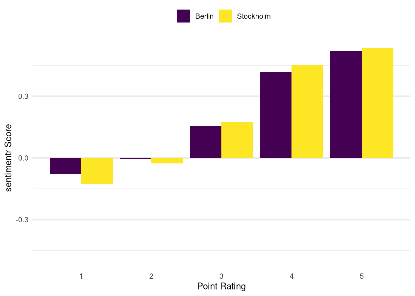
We still observe the same qualitative pattern as with the simple lexicographical approach: The point score is positively correlated with the sentiment score in within cities.
Also the scores from Stockholm are still more pronounced than the Berlin scores in each category but the relative difference is much lower than with our previous calculations. This might be an indication that the differences we saw previously were partly caused by the inability of the lexicographical approach to handle the negations and amplifiers correctly or the presence of more descriptive text in the Berlin data.
A Neural Network Model
The two methods we have presented so far can be regarded as heuristic as both
the scoring of the individual words in the lexicon as well as the structure and
coefficients of the equation in the sentimentr package are first and
foremost based on human assessment.
We will now turn to supervised machine learning methods as an alternative paradigm to produce a sentiment score. This approach still requires human assessment in the form of labels that determine whether a text contains a negative or positive. However, once these labels have been established it will be up to the model’s training algorithm to describe the relationship between the sentiment label and the input text based on the data it processes.
For our review data we do not have the sentiment labels available to train our own model (in fact these labels are what we are trying to obtain) but luckily there are frameworks available that provide pre-trained models for sentiment analysis. One such framework is the flair package which provides easy access to state-of-the-art machine learning models for NLP (Natural Language processing) tasks.
In many areas of machine learning research the state-of-the-art models nowadays tend to be neural network models and this definitely is the case for Natural Language Processing (NLP) problems.
Neural networks have the ability to
approximate any kind of function
which makes them very suitable to represent the complex structures that can arise
in textual data and in our case we are interested in describing the functional
relationship between the raw input text and the associated sentiment. If we
allow the model enough complexity and training time it will build representations
of the input texts that will enable it to identify structures that indicate
negative or positive sentiments (such as negations or amplifiers). This means it
will derive rules similar to those encoded in the equation of the sentimentr
package by itself.
While the power of neural networks is indisputable they do have some disadvantages. One of them is the fact that it is extremely difficult to understand how the network arrives at its predictions. It may building decision rules similar to the heuristics we have described above but translating these rules into a form that a human can understand them is not necessarily possible.
Another drawback is that neural networks tend to be extremely computionally expensive which is why in practice specialised machines are often used when working with neural networks.
As a matter of fact the computational requirements made it impractical for us to use the more advanced transformer based neural network in the flair package and instead we had to use the somewhat simpler recurrent neural network (RNN) that allowed for reasonable computation times on my machine.
The model we used was trained on a dataset consisting of movie and product reviews where each text was assigned a negative or positive label. Therefore the output from the model is the estimated probability that a given piece of text expresses a negative or positive sentiment. This is an important difference from our previous approaches where the score was an expression of the strength of the sentiment. We will need to keep this in mind when interpreting the results of the model.
For our analysis we took the output from the model and scaled it such that a value of -1 corresponds to a 100 % probability of a negative sentiment and +1 to a 100 % probability of a positive sentiment. A score of 0 means that the model is undecided about which sentiment to assign.
Using this approach the resulting distribution of sentiment scores looks as follows:
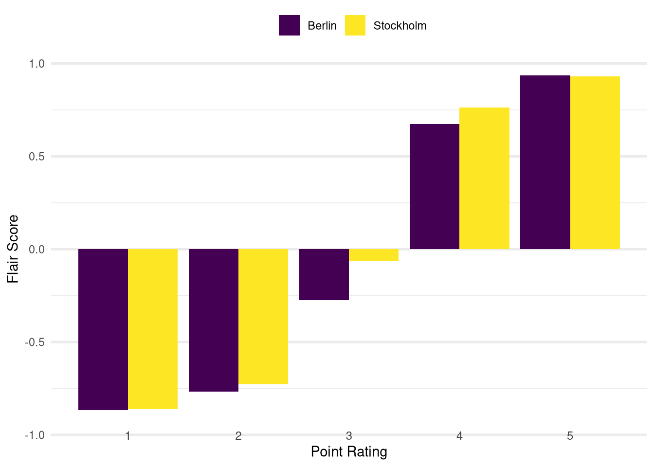
As in the cases before the distribution for both cities follow the same pattern in the sense that higher point ratings are associated with higher sentiment scores (and vice versa for lower point ratings).
Again we focus our attention on comparing the sentiment scores between the two cities to answer our initial analysis question for this blog post: We can see that the scores from the neural network reproduce the positive difference between the scores from Stockholm and Berlin in the four point category. While the difference seems to be relatively smaller than what we saw with the previous methods this can still be regarded as evidence to support our subjective observations that motivated this analysis.
Interpreting the Neural Network Scores
Apart from that the scores from the neural network differ quite a bit from the previous methods: On the one hand the sentiment scores from Berlin now have higher magnitude than the ones from Stockholm (the four point category being the only real exception as mentioned above).
Also the distributions for both cities are now much more symmetric in the sense that in the low point categories the scores have almost the same magnitude as in the high point categories (just with reversed signs). The previous distributions were much less symmetric with skews towards higher scores.
To understand those differences we need to remind ourselves that the metric produced from the neural network is not a measurement of the strength of sentiment but reflects the certainty of the model about whether a given text expresses a positive or negative sentiment.
Therefore the fact that the absolute magnitude of the scores in the one point and five point category are almost the same does not imply that the sentiments expressed in those categories are equally strong. It simply means that the model is approximately equally sure about the cases in those rating groups reflect negative and positive sentiments respectively. Intuitively a relationship between this measure of certainty and the strength of the sentiments is plausible but we have no justification to simply assume it exists.
In general the model seems to be quite confident in its predictions, which can be confirmed by looking at a histogram of the its predictions:
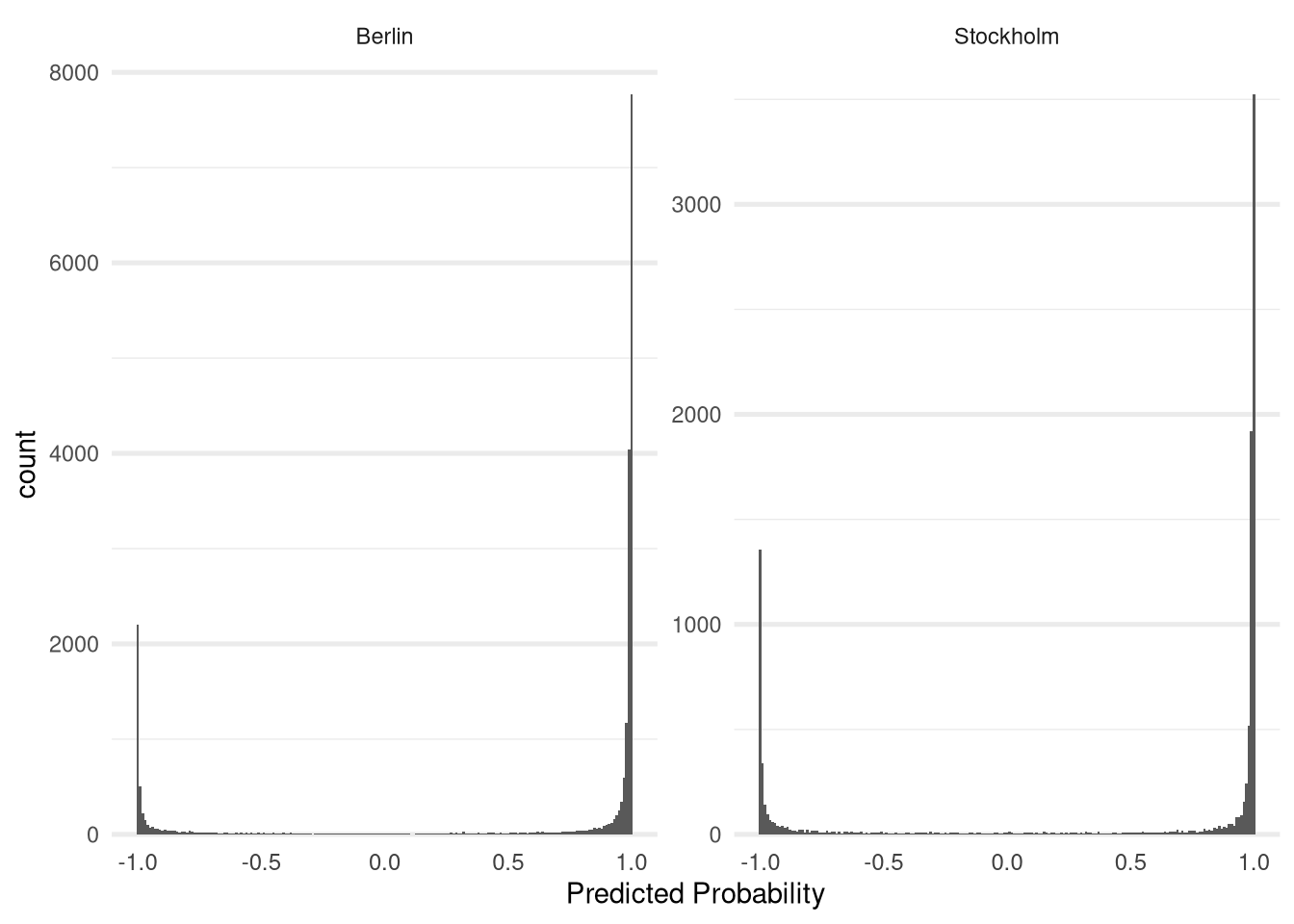
The distribution of the predicted probabilities is heavily focused on the extreme ends of the spectrum for both cities.
As we already mentioned above it is difficult to understand how a neural network arrives at its predictions. One thing we can do though is to look at some of its predictions and the associated input text to get an idea of what it might be doing. This might be especially useful to identify cases with which the model seems to struggle.
For example, the following reviews all got a highly negative score but obviously seem to express rather positive sentiments:
“I can only recommend it”
“Great for business lunches, but also for dining out with friends. On request there are always vegetarian delicacies and I don’t know of any place in Berlin where a steak is cooked better to the point. The service is second to none. I can only recommend it!”
It’s very nice .. Amazingly cheap 🤷♂
The upper hammer! Unfortunately not cheap, but seriously, the evening was worth every penny.
The occurrence of the phrase “I can only recommend it” in the first and second review make you wonder whether there might be an issue with that particular phrase that leads to the low scores.
The special characters in the third example might have caused issues in the preprocessing step before passing the data to the model.
The results for the fourth example may be affected by the improper translation of the positive German slang word “Oberhammer” but should probably still result in a much higher score.
It is also possible to find some examples which are off in the opposite direction, such as the following review which received a score of 0.95:
Have to wait a long time for food.
We also spotted some examples where mild criticism within a generally positive review seems to be overemphasised leading to a low score:
“Good treatment fresh premises … The pizza was good but the Pepperonin was strong.”
“Convincing cuisine at fair prices. Tell the cook: Please spicy, then it will be even tastier! The lamb was better than the chicken by the way …”
These two reviews have a score of around 0 and -0.38 respectively which seems too low compared to some of the other predictions of the model.
It should be pointed out that we don’t claim the cases above should not be viewed as representative examples of the model’s performance in general. While performing the face validity checks on the model’s predictions those cases were definitely the exception rather than the norm. We should also keep in mind that the model was not trained on restaurant reviews specifically and might therefore be insensitive to a lot of the specific lingo (such as descriptions of taste or atmosphere).
However, we should use these examples as a reminder that even state-of-the-art neural network models are not infallible, especially when we are applying a pre-trained model on data that is not necessarily comparable with the data it was trained on.
Conclusion
In this blog post we presented and applied three different methods to analyse the sentiments in restaurant reviews from Stockholm and Berlin. Each of the method showed a difference in the sentiments within the category of ratings with four points which we can interpret as evidence to support our subjective findings that motivated this analysis. However, we should be cautious to lean on these findings too much as all the methods we applied have their limitations as we pointed out during the course of the analysis.
In our next post we will further explore the relationship between review texts and the point score by building and analysing models that predict the point rating from a given review text.