Welford’s Algorithm for Calculating Variance

A colleague suggested we should go with a different approach and introduced us to Welford’s algorithm. Welford’s algorithm is an online algorithm which means that it can update the estimation of the sample variance by processing one observation at a time.

This approach has the distinct advantage that it does not require you to have all the observations available to update the estimations of mean and variance when a new observation comes in.

To make this a bit more clear, below is the formula which you would normally use to calculate the variance from a set of observations \(x_1,\dots, x_n\):

\[s^2_n = \frac{\sum_{i=1}^n (x_i - \bar{x}_n)^2}{n-1}\]

Here \(\bar{x}_n\) denotes the sample mean \(\frac{1}{n}\sum_{i=1}^n x_i\).

To calculate the variance using this formulation it is necessary to have all the observations \(x_1,\dots,x_n\) available at any time. In fact you have to go through the whole dataset twice: once to calculate the mean \(\bar{x}_n\) and then another time to calculate the variance itself. Therefore this formula is also referred to as the two-pass algorithm.

The idea of Welford’s algorithm is to decompose the calculations of the mean and the variance into a form that can easily be updated whenever a new observation comes in.

For the mean this transformation is produced by simply rewriting the formula for \(\bar{x}_n\) as the weighted average between the old mean \(\bar{x}_{n-1}\) and the new observation \(x_n\):

\[\bar{x}_n = \frac{\sum_{i=1}^n x_i}{n} = \frac{\sum_{i=1}^{n-1} x_i}{n} + \frac{x_n}{n} = \frac{(n-1)\bar{x}_{n-1} + x_n}{n} = \bar{x}_{n-1} + \frac{x_n - \bar{x}_{n-1}}{n}\]

The decomposition for the variance is slightly more complicated. Only looking at the enumerator (the sum of squares of differences) of the formula for \(s^2_{n}\) from above we can derive it in the following way:

To get the variance we just need to divide the formula above by \((n-1)\) which yields:

\[s^2_n = \frac{n-2}{n-1} s^2_{n-1} + \frac{(x_n - \bar{x}_{n-1})^2}{n}\]

The derivation above shows that the updating formula is algebraically equivalent to the standard formula for variance presented in the beginning of this section.

However, the new formulation has the distinct advantage that it does not require all of the observations to be available at computation time but instead can be used to sequentially update our estimation of the variance as new data comes in. At any point in time our algorithm only depends on four values as input:

• the observation \(x_n\)
• the total count of observations \(n\)
• the current estimate of the mean \(x_{n-1}\)
• the current estimate of the variance \(s_{n-1}^2\)

In practice it is preferable to keep track of the sum of squares of differences \(M_{2,n} = \sum_{i=1}^n (x_i - \bar{x}_n)^2\) instead of the variance \(s_n^2\) directly due to numerical stability considerations. Doing so results in the slightly different formulation which is presented in the Wikipedia article and which we will be using in our analysis as well.

Discrepancies Between Welford’s Algorithm and Standard Formula

The fact that Welford’s algorithm and the standard formula for variance estimation are algebraically equivalent does of course not guarantee that they will always produce the same values when they are implemented in a piece of software as many potential sources of errors can occur. An obvious example that comes to mind is human error in implementing the solution but there are also more subtle things such as numerical issues that arise when doing arithmetic with limited floating point precision.

While testing the results of the real-time outlier detection algorithm against an offline implementation that was previously run manually by data analysts some discrepancies between the two solutions were detected.

We were able to trace back the differences in the results to discrepancies in the estimates for the variances. Since for our practical purposes the differences were negligible (relative errors on the scale of maybe up to \(1-5\%\)) and tended to result in a slightly more conservative behaviour of the online algorithm (which was acceptable in our use case) we decided not to analyse the issue any further.

Simulation Study

We assumed that the discrepancies we saw originated from inherent differences between the variance estimation in the two algorithms (the offline solution used the standard variance formula). However, after doing some superficial research into the issue it seemed unlikely that with the data we had on our hands the two estimations should differ from each other as much as they did in our test.

Intuitively it seemed more likely that other differences between the two implementations were the real cause for the differences we witnessed (e. g. the way the data was stored and retrieved or a subtle bug in either of the implementations).

Since I don’t have access to the original data or the implementation anymore I decided to do a little simulation study using real world datasets to see if I could replicate discrepancies similar to the numbers we saw in our analysis.

As done previously in the linear regression post we will use datasets from the OpenML dataset repository. Instead of R we will be using Python this time as this is the language the original implementation was done in.

To run the simulation we will use Metaflow which is a framework for automating data science workflows, originally developed by Netflix but now released as open source software.

Metaflow has a lot of nice features, such as seamless integration with AWS services but for our simulation study the most important advantages are the built-in data management which make the analysis of our results much easier as well as the automatic parallelisation that will greatly speed up the runtime of our simulation.

The code for the Metaflow implementation can be found here. Using an appropriate Python environment the simulation can be started by simply running the following command in the bash:

python welford_sim_flow.py run --random_seed=4214511 --num_datasets=500 --max_obs=10000000 --max_cols=20 --max_cols_large_datasets=5 --n_def_large_datasets=100000 --max-num-splits=500

The definitions of the command line parameters their definitions can be looked up in the source file of the flow.

The Metaflow run will output status messages with information about the progress of the simulation:

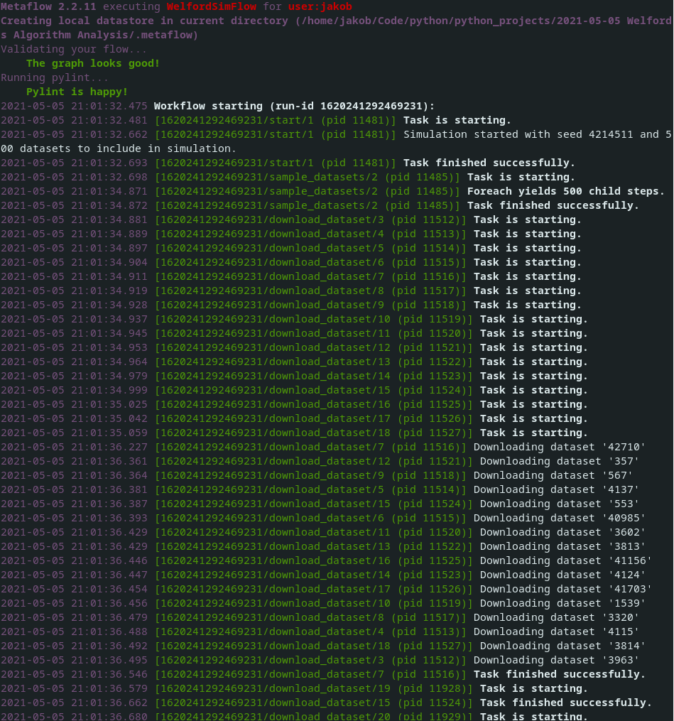
The individual steps of the process, their execution in parallel as well as the transfer of the data between them are completely managed by Metaflow.

Metaflow will persist the results of the simulation run (in our case in a local folder .metaflow/ in the same directory as the code files) which can easily be accessed from a Jupyter Notebook using the Metaflow client API. You can see how this is done in the Jupyter Notebook file containing the code to reproduce the results presented below.

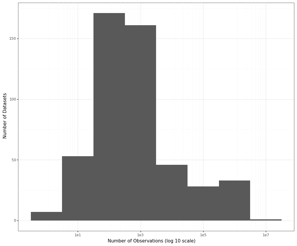
For our analysis we sampled 500 datasets from OpenML ranging between 2 and 4,898,431 observations each with the median number of observations per dataset being 400.

The plot below shows the distribution of the sample sizes of the datasets on a log (base 10) scale:

For each dataset a subset of the numerical columns was sampled and for each of these columns we calculated the variance twice: once using the implementation from NumPy (to represent the standard variance calculation formula) and the other time going through the data sequentially using Welford’s algorithm.

Overall we produced 7935 pairs of variances this way and measured the deviation between the two by calculating the relative errors (relative to the NumPy variance estimates).

The distribution of the relative errors is shown in the plot below (note the log scale on the x-axis):

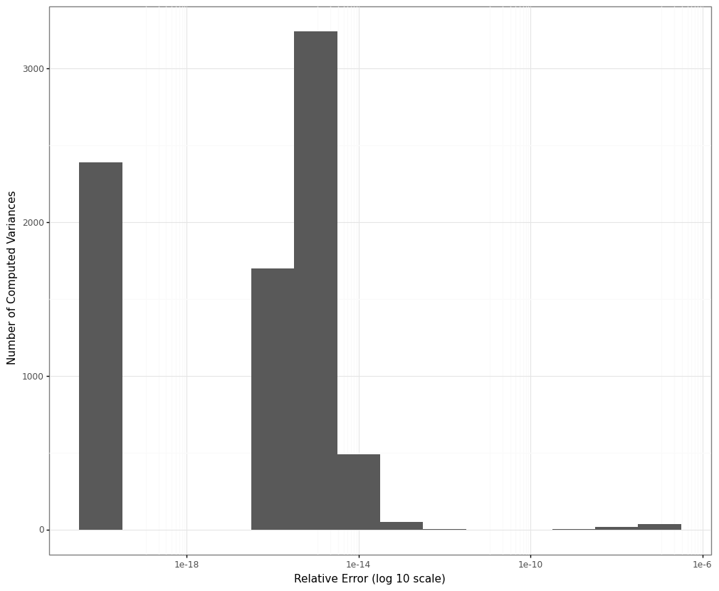
To make sure all the relative errors could be calculated and plotted we shifted both variance estimates and the relative error numbers by a value of \(10^{-20}\). Therefore the values in the bucket of relative errors of \(10^{-20}\) are corresponding to cases in which the two variance estimates matched exactly. Those cases made up around 30 % of all our simulation results.

The maximum relative error we observed was on the order of magnitude of \(10^{-7}\), the mean and median relative errors turned out to be around \(4.9\cdot10^{-10}\) and \(2.9\cdot 10^{-16}\) respectively.

The relative errors we obtained in our simulation are therefore much lower than the ones we observed during the test of the fraud detection algorithm which motivated this analysis (the relative errors we saw there were on the scale of \(\approx10^{-2}\)).

It could well be that none of the datasets included in our simulation had the same characteristics as the data that produced the larger relative errors in our previous analysis. The real-world data that was used in that test tended to be approximately log-normally distributed. However, running a number of simulated observations from various log-normal distributions through our simulation setup described above also failed to replicate relative errors on that scale.

So while we can not rule out that the original discrepancies were caused by inherent differences in the calculations of the variance it now seems much less likely.

As already mentioned I do not have access to the code or the data anymore but I would guess that the differences were caused by subtle differences in the implementations. Especially the fact that the variables necessary for the Welford updates (\(M_{2,n}, \bar{x}_n, n\)) were stored in a MySQL table with limited floating point precision may be an issue.

Theoretical Analyses

Aside from the results of our simulations it is worthwhile to look at some more theoretical analyses of the behaviour of the variance estimation methods.

In particular this paper by Chan et al from 1983 (which is also referenced in the Wikipedia article) and this blog post by John Cook.

Both articles investigate which algorithm best approximates the true, known variance of simulated samples (whereas our analysis focused on whether they differ from each other without making any claims which of the two is more precise).

The Chan paper presents an overview of different algorithms for calculating the variance and points out some potential problems with some of them. In particular they derive theoretical bounds for the errors one can expect with each of the methods depending on the sample size, machine precision and the condition number of the dataset \(\kappa\) (a measure of how sensitive the variance estimation is to the data it encounters). They also validate their theoretical bounds in a simulation study (using sample sizes of \(N=64\) and \(N=4096\)).

Interestingly their findings suggest that Welford’s algorithm yields comparably higher error rates than most of the other candidates (out of which the one referred to as two-pass with pairwise summation in the paper might be the closest match for the variance estimation from NumPy).

However, some of the findings and recommendations in the paper seem a bit out of date as most toolboxes for numerical calculations nowadays use many of their recommendations for improvements as default (e.g. pairwise summations to avoid rounding errors). Therefore it might be difficult to translate their findings to modern implementations.

A more up-to-date analysis of the accuracy of Welford’s algorithm is the blog post by John Cook (which is actually part three in a series of posts). In it he compares how well Welford’s algorithm and the standard formula (which he refers to as the direct formula) approximate the theoretical variance of some simulated observations. Based on his C++ implementation he concludes that both formulas perform similarly well, even giving Welford’s algorithm a slight edge.

In his analysis he is also able to generate datasets in which the two algorithms deviate both from the theoretical variances as well as with each other up to a certain set of digits. However, the cases he presents consist of relatively small numbers (sampled from a uniform distribution between zero and one) shifted by huge values (up to \(10^{12}\)). These results are definitely interesting and theoretically valuable but they should not be helping us to explain the discrepancies we saw in our outlier detection scenario where the data tended to be much more well-behaved.

Conclusion

In our analysis we compared the results of two different ways of calculating the variance based on a simulation with 500 datasets. We concluded that the discrepancies between them lie in a range which makes them interchangeable for most practical applications. In particular we were not able to reproduce any discrepancies on the order of magnitude that were seen in a previous implementation which motivated this post, hinting that these results were probably caused by some other implementation difference.