Modelling the Relationship Between Restaurant Review Texts and Point Ratings
In our last post we used sentiment analysis to find out whether there is a difference in the relationship between the wording of restaurant review texts and the associated point score between Stockholm and Berlin.
Today we will revisit this subject using a different approach. We will fit statistical models to our data to formalise the relationship between the review texts and the associated point ratings.
We can then use the predictions and coefficients of these models to answer the following question:
Is a review text of a five point rating from Berlin likely to receive a lower rating in Stockholm?
A positive answer to this question can be regarded as supporting evidence for our subjective observation that there are many review texts in Stockholm corresponding to reviews with less than five points that would have received the full five point rating in Berlin.
Modelling the Target Variable
For this analysis we will fit logistic regression models which are used to classify observations into two distinct classes. In our case these two classes will be the five point reviews (which we will also refer to as the positive class) and the reviews of less than five points (the negative class).
It should be noted that for data on a fixed scale that has a meaningful ordering (such as the point ratings we are dealing with) it would be more appropriate to use an ordinal regression model. Since for our analysis however we are only interested in the distinction between five point ratings and ratings with less than five points we will go with the simpler logistic regression model.
Building Numerical Features from the Review Texts
One of the key ingredients in our model building process is the way we transform the review texts to numerical data that can be used as predictor variables in our models. For our analysis we will fit three types of models whose main differences lie in how this transformation is done.
For the first model we will use a simple bag of words type transformation to generate the features. Using this approach the the text data is converted into a vector in which each entry corresponds to a word (or combination of words) from a predefined list (the dictionary). The entry will be zero if a given word is not present in the review text and have a value different from zero if it is (e.g. it could be \(2\) if the word occurs two times in the text).
Arranging these vectors into rows will produce the document term matrix (DTM) in which each row corresponds to one review text and the columns to a word or word combination. This matrix along with the target variable described in the previous section will be used to fit our logistic regression model.
The process to create the DTM is a bit more complicated than described above and
involves, for example, the removal of certain unimportant words or words that occur
too rarely to make any difference in the model. In our implementation (which can
be found
here)
we used the text2vec package and followed the steps outlined in its
vignette.
We deviated from the recommendations in the vignette with respect to one important aspect: Instead of the TF-IDF transformation we applied the simpler L1-normalisation that converts the word counts into the relative frequencies with which a given word occurs in a text.
The reason for that is that the TF-IDF transformation includes factors that are calculated from the whole dataset. Therefore its results will vary depending on which dataset the transformation is applied on. This is an undesirable property for our purposes as in the next section we will fit two separate models: one on the data from Berlin and one on the data from Stockholm. We then will use both models to predict on data from Berlin
However, this can only be done if the features we put into the models have been calculated in the same way for both datasets. This is not the case for the TF-IDF normalisation which will produce different values for the same review text, depending on which dataset it is in.
The L1 normalisation on the other hand can be applied independently on each observation and therefore will produce compatible predictor variables.
Regularisation for Feature Selection
The model we will fit is a logistic regression model with lasso regularisation (L1). This means that during the training process an additional penalty term is introduced into the objective function that will prevent the model from fitting too many coefficients. As a result we will end up with a model with less (non-zero) coefficients which will be easier to interpret and analyse. This is a big advantage as our models will tend to have many potential predictor variables (the models in the next section will have 2893 potential predictors).
How much the model is being penalised for fitting non-zero coefficients (i.e. the strength of the regularisation) will be automatically chosen as a hyperparameter during the training process using cross validation.
Separate Models for Each City
Our first approach to formalise the relationship between the review text and the point ratings in the two cities will be to fit one model for each city separately.
To be precise the models for each city will fit the linear relationship between the log-odds \(l\) of an observation being a five point review and the predictor variables. This relationship can be written down as:
\[l = log(\frac{p}{1-p}) = \beta_{0} + \beta_{1}\cdot X_1 + \dots + \beta_{n}\cdot X_n \]
In this formulation
- \(p\) refers to the probability of an observation being a five point review
- \(\beta_{0}\) refers to the intercept of the model (which incorporates the “average” probability of a five point review)
- \(X_{i}\) is the value for the i-th word or n-gram as encoded in the document term matrix
- \(\beta_{i}\) is the coefficient for variable \(X_{i}\)
Our main quantity of interest will be the values that our models predict for \(p\) which can be recovered by a simple transformation of the log-odds.
The models for each city share the same model formulation but since we will fit them on different datasets (the data from the respective city) they will have different coefficients.
Effect of the Intercept
In our first post about the restaurant reviews data we saw that there is a big difference in the proportion of five point reviews between the two cities: around 47 % in Stockholm vs about 64 % in Berlin.
This will present a problem for our separate models approach which can be see when passing some example review data through each of the two models:
## # A tibble: 6 x 3
##   review_text                                       Berlin_model Stockholm_model
##   <chr>                                                    <dbl>           <dbl>
## 1 "This is a great restaurant, I really enjoyed th…        0.902           0.742
## 2 "One of the best restaurants I have ever been. A…        0.947           0.940
## 3 "The staff is super friendly and the food is mag…        0.927           0.760
## 4 "If your looking for the best food in town, this…        0.842           0.791
## 5 "Had a brilliant time here with my family. The f…        0.889           0.785
## 6 ""                                                       0.677           0.432
For most of these example reviews the predictions for a five point review from the Berlin model are considerably higher than from the Stockholm model (on average around 12 %) and we might be inclined to read this as substantial proof towards our research hypothesis.
The problem becomes clear when we look at the last example review which is just an empty text string. Even for this data the Berlin model predicts a 24.5 % higher probability for a five point review. This property of our models is certainly undesirable when we want to analyse how a given review text might result in a different point ratings.
The reason for this issue is that logistic regression models are fit in such a way that the average prediction will be approximately calibrated to the proportion of the positive class. Since this number is higher in Berlin than in Stockholm, so will be the predictions of the Berlin model, even on an empty text. This issue manifests itself in the intercept term \(\beta_0\) in our models and makes the comparison of the predictions difficult.
We can remedy the situation by artificially giving the five point reviews in Stockholm more weight during the training process so that their proportion will be the same as in Berlin.
By doing so the average predictions of the two models will have the same level and the difference between their predictions will have a more meaningful interpretation for our analysis:
## # A tibble: 6 x 3
##   review_text                            Berlin_model_corre… Stockholm_model_co…
##   <chr>                                                <dbl>               <dbl>
## 1 "This is a great restaurant, I really…               0.902               0.863
## 2 "One of the best restaurants I have e…               0.947               0.953
## 3 "The staff is super friendly and the …               0.927               0.883
## 4 "If your looking for the best food in…               0.842               0.865
## 5 "Had a brilliant time here with my fa…               0.889               0.870
## 6 ""                                                   0.677               0.672
With the reweighting the two models now give very similar predictions on the empty review texts. Also the big differences we saw previously on some of the other example texts have now gone down substantially and in some cases even reversed.
Differences in Predictions Between the Two Models
Now that we have two comparable models we query them to try and answer our initial question about whether five point ratings from Berlin are less likely to receive a five point score in Stockholm.
For this we simply run the five point reviews from Berlin through both of the models in the same way as we did for the example reviews above and analyse the differences in their predictions.
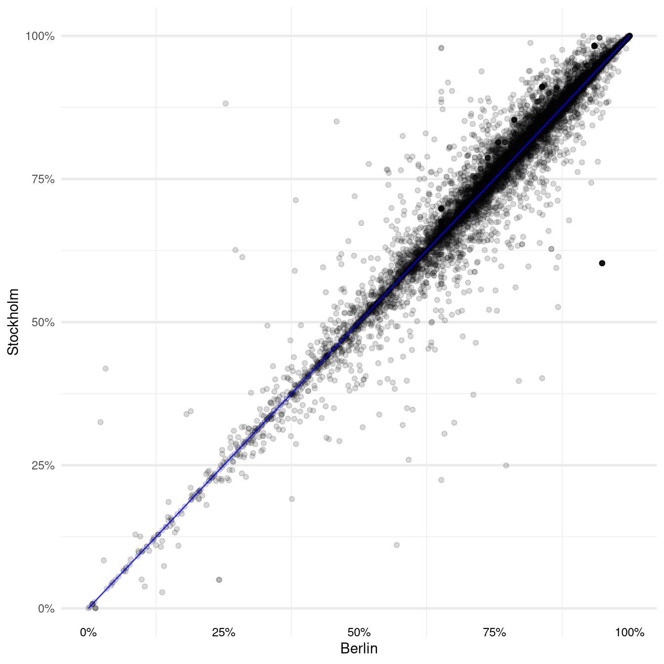
We can get a visual impression of the overall difference by plotting the resulting predictions against each other in a scatter plot:
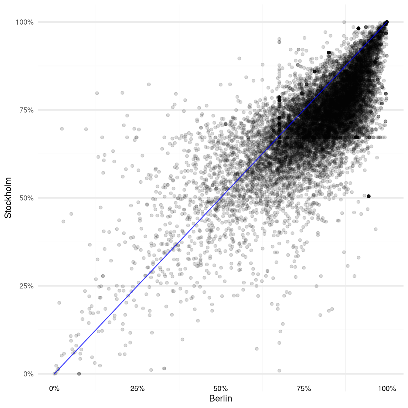
Each point in this plot corresponds to a five point review from Berlin. Its location on the x-axis is determined by the predicted probability for a five point rating according to the Berlin model and its position on the y-axis corresponds to the probability for a five point rating assigned by the Stockholm model.
This means that for all observations that are plotted below the blue identity line the Berlin model is predicting a higher probability than the Stockholm model.
It is a bit hard to make out but the concentration of points in the upper right quadrant of the plot might suggest that overall the average predictions from the Berlin model are higher than the Stockholm model.
And indeed this is the case: The average difference across all the five point reviews from Berlin turns out to be about 6.6% which seems to validate our subjective impression.
Analysing the Coefficients
Another interesting pattern in the plot are the vertical and horizontal lines of points that meet around the coordinate \((67 \%, 67 \%)\). These are formed by observations for which either the Berlin model (vertical line) or the Stockholm model (horizontal line) only predict the intercept probability. This means that the corresponding review texts did not contain any words that have a non-zero coefficient in the respective model.
In general it will be interesting to have a closer look at the coefficients of the two models to understand how they arrive at their different assessments and which pieces of texts are informing their prediction.
First let’s look at the coefficients that have high positive or negative coefficients in both models:
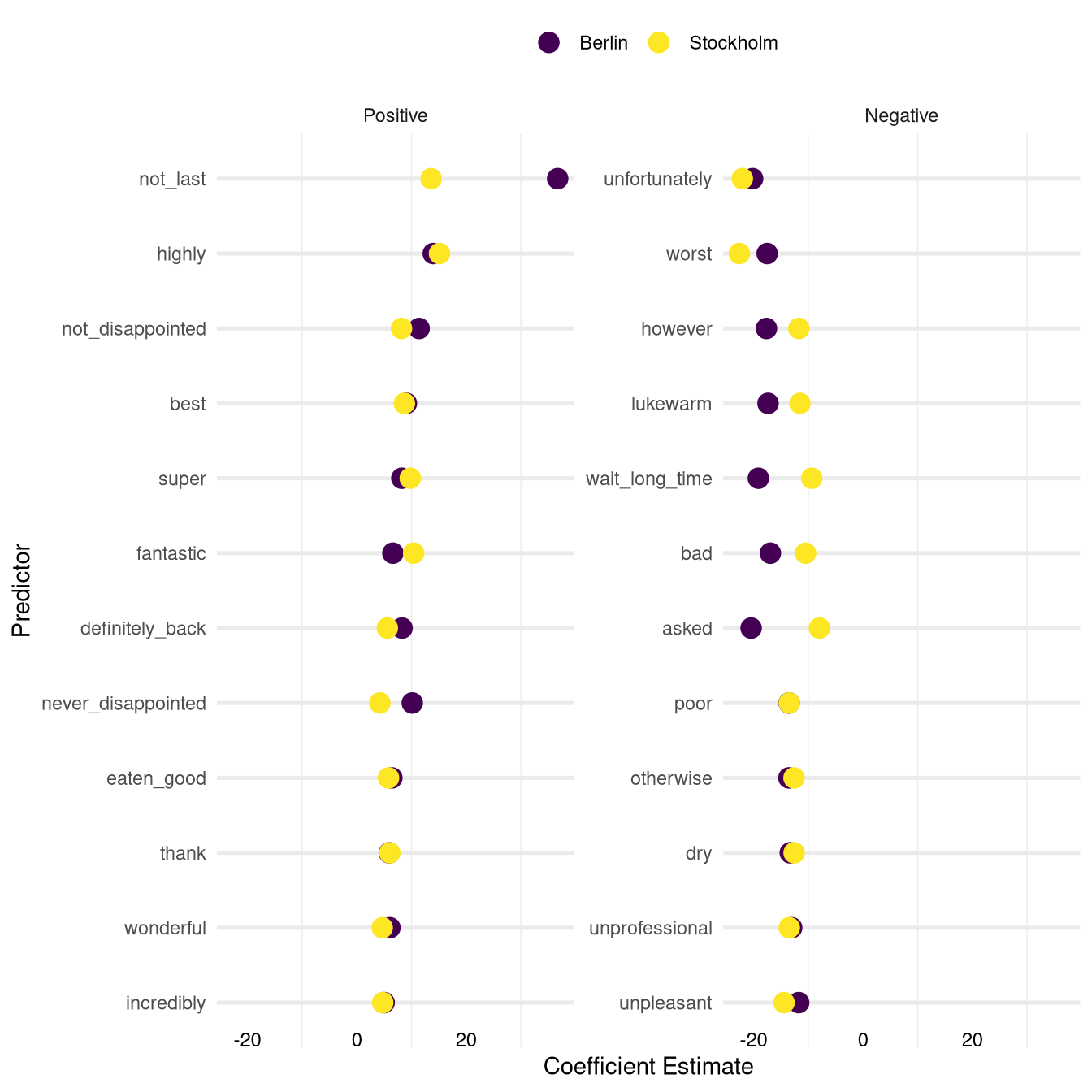
The plot above shows the coefficients which have a high positive (left panel) and a high negative (right panel) coefficient in both models. They have been selected by sorting the coefficients for both models separately and calculating the average rank between the two models.
Note that certain stop words (such as the, we, had, to, etc.) were removed from the text before generating the text features. Therefore expressions such as wait_long_time refer to pieces of texts that originally read something like “we had to wait a long time” or similar.
All of the words and phrases on the two lists intuitively make sense: you would expect their presence in a review text to have a strong positive or negative impact on the probability of a five point review.
This is a good sense check for our model. The only two entries on the list which might raise our eyebrows are the words however and otherwise. But it is plausible to assume that they are frequently used in qualifying statements in which users explain why they did not give the full five point score (e.g. “We had a good night however the noise level in the restaurant was uncomfortable”).
On the left side we see a lot of overwhelmingly positive words as well as expressions of fulfilled expectations (not_disappointed, never_disappointed). Also phrases of intent to return to the restaurant seem to have a high positive impact on the probability of a five point review (not_last, definitely_back).
On the negative side we can see some specific criticism of certain aspects of the restaurant experience (wait_long_time, unprofessional) or the food (dry, lukewarm) mixed in with some more general negative expressions (bad, poor, worst, etc.)
Now let’s look at the coefficients on which the models disagree. The lists below contain coefficients that have either highly positive or negative coefficients in the Berlin model but values of zero (indicating no effect) in the Stockholm model:
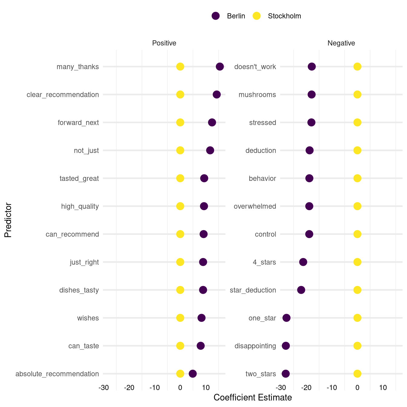
One thing that stands out on the list on the left side is the presence of words and phrases referring to the taste of the dishes ( can_taste, tasted_great, dishes_tasty). Another cluster can be formed around expressions involving the word recommend (clear_recommendation, can_recommend, absolute_recommendation).
On the negative side we have a lot phrases that refer to the point rating the user is giving ( one_star, two_stars, 4_stars, star_deduction, deduction) for which a strong negative impact on the probability for a five point rating is very plausible.
A lot the other negative factors that might lead to a low rating in Berlin seem to revolve around the service ( unfriendly, overwhelmed, behavior, stressed).
A curious entry on the list is the word mushrooms which could be interpreted in different ways (maybe there is a high frequency of bad mushrooms in Berlin restaurants or a tendency to ignore customers’ requests to exclude mushrooms from their meal).
Finally let’s look at the coefficients that have high impact in the Stockholm model but no impact in the Berlin model:
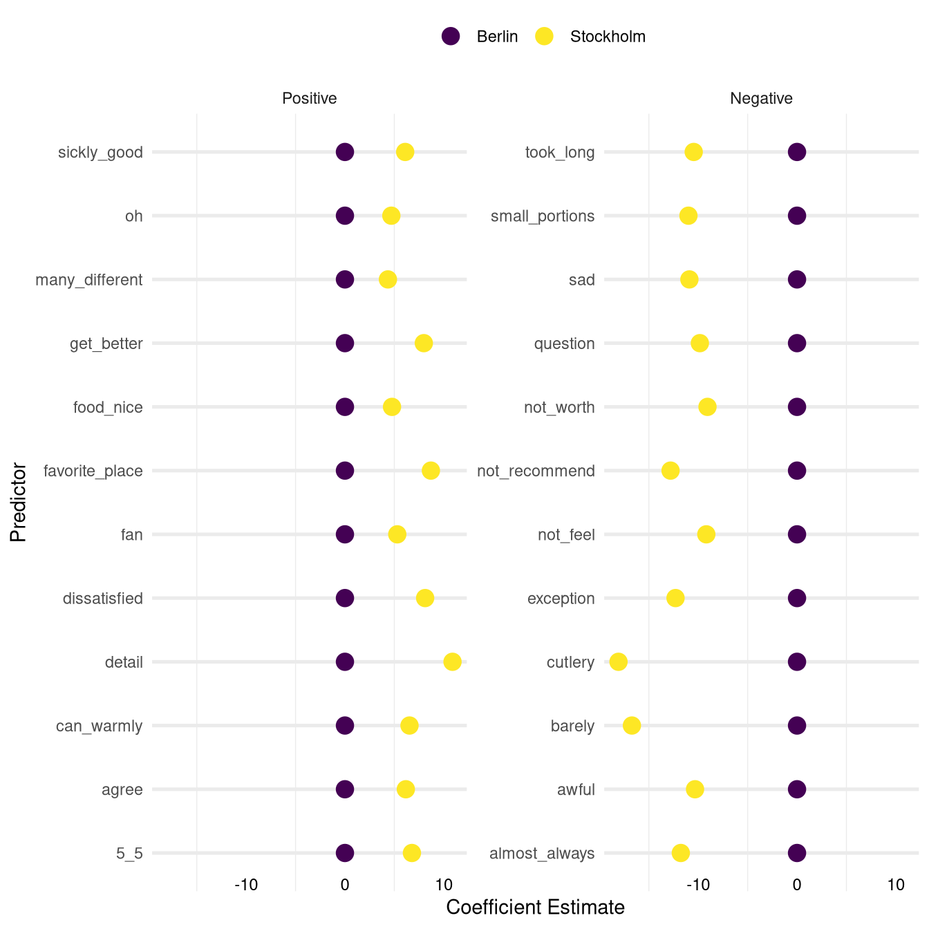
The list of positive coefficients in Stockholm seems to consist of a mixed bag of positive expressions with no clear unifying topic.
The entry sickly_good looks like it might be the result of an improper translation of a Swedish idiom.
In addition to that it is not immediately clear why the word dissatisfied pops up on the list of the positive coefficients.
On the negative side the entries took_long, small_portions and (curiously) cutlery describe very specific aspects of the restaurant experience that seem to be important for users in Stockholm. Apart from that the list contains a lot of generic negative statements such as awful, not_recommend, or not_worth.
Limitations of the Bag of Words Features
In our analysis of the coefficients above we have found some interesting differences between the two models and we might be tempted to generalise them into statements outside the realm of model analysis.
While these generalisations are always extremely difficult and require a thorough understanding of the data generating process, they are especially difficult to make with the models we have built as we will see below.
For example, we could be inclined to translate the fact that the coefficients for tasted_great, dishes_tasty, and can_taste are highly positive in the Berlin model but zero in the Stockholm model into a bold statement such as the following:
People in Stockholm do not care about the taste of their food (but people in Berlin people do).
Even if the sample of restaurant reviews that we used to train our model was in theory good enough to make these kind of inferences (which it probably is not in our case and in general rarely ever is) we should remind ourselves about how exactly we constructed the features we used in our model from the raw review texts.
As described above the simple bag of word features we are just counting with which frequency a word appears in a given text. The important point to stress here is that the variable will only account for the presence of an exact word or phrase.
So while it may be true that the exact expression great_taste is not important in the Stockholm model, it may well be the case that other positive descriptions of food taste are important. And in fact the expressions tastiest and fresh_tasty are examples of coefficients that have positive values in the Stockholm model while they are zero in the Berlin model.
Therefore we have to be aware that the validity of our analysis is largely influenced by the compatibility of the vocabularies used in the reviews from the two cities. If there is a tendency to describe the same issues with different words or expressions this will pose a problem.
This issue is especially relevant in our case since we are working with review texts that were machine translated from Swedish and German to English. Words with very similar or identical meaning could be translated to different words in English as can be seen in the example below:
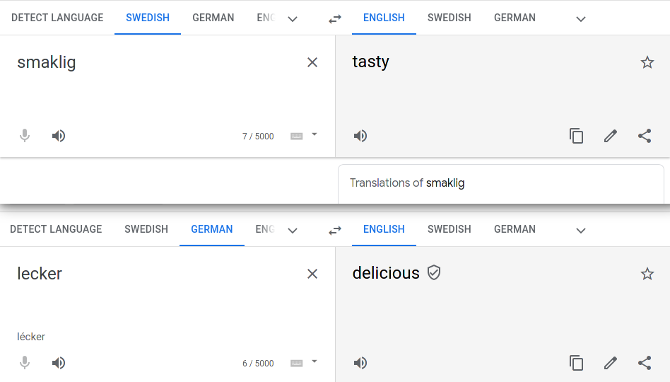
Even though the two original words basically have identical meaning they will be encoded in separate variables with no way for the model to make any connections between them.
Ideally we would want to use features in our model that go beyond the simple counting of words in a text and are powerful enough to encode semantic information and relationships in different pieces of text.
This will make the comparison of the two models more meaningful and also improve the predictive performance of the models themselves as the data can be used more efficiently.
Unified Model
Luckily, these kind of features do exist and we will use them in our final model in the next section. But first we will revisit our modelling approach.
While intuitively it makes sense to build two separate models, each describing the rating process in the two cities separately, it may not be the most elegant or standard approach.
An alternative way to approach our problem is to formulate one single, unified model which we train on all the data and explicitly use the coefficients of the model to describe the differences between the two cities.
Such a model could be formulated in the following way:
\[l = \beta_{0} + \beta_{0,city} \cdot X_{city} + \beta_{1}\cdot X_1 + \dots + \beta_{n}\cdot X_n + \beta_{1,city}\cdot X_1 \cdot X_{city} + \dots + \beta_{n,city}\cdot X_n \cdot X_{city}\]
The coefficients and variables \(\beta_0\), \(\beta_{i}\) and \(X_i\) have the same meaning as in our previous formulation.
The key difference compared to our previous model is the introduction of the city dummy variable \(X_{city}\). For the data from Berlin this variable will have a value of zero and therefore the model will reduce to our previous model’s formulation.
For data from Stockholm on the other hand the value of \(X_{city}\) will be \(1\) which means we will use that data to fit the additional coefficients as offsets from the Berlin data.
The city specific intercept \(\beta_{0,city}\) will describe the difference in the overall incidence of five point reviews between Stockholm and Berlin. Therefore this variable will capture the difference we have previously accounted for by reweighting which we can now drop (we will just have to make sure we use the same intercept when measuring the prediction differences).
The other additional coefficients \(\beta_{i,city}\) describe the interaction between the city dummy \(X_{city}\) and our word feature variables \(X_i\). This means they will describe how the effect of a given word on the probability for a five point review differs between Stockholm and Berlin. For example, if the word \(i\) has a more positive effect on the rating for reviews from Stockholm than in Berlin the coefficient \(\beta_{i,city}\) will be positive.
This formulation also makes the analysis of coefficients much simpler as we can simply look at the offsets \(\beta_{i,city}\).
The coefficients \(\beta_{i}\) are also called the main effects and the coefficients \(\beta_{i,city}\) are referred to as the (city-)interaction effects.
Fitting a model as described above is a bit more complex, especially when working
with the glmnet package as we will have to build the design matrix which encodes
the data for the logistic regression model manually. If you are interested in how
this is done exactly please check out the code here.
Results From the Unified Model
As we have done before we will estimate the difference in the text to rating relationship by looking at the differences in predictions on the five point ratings from Berlin.
To obtain these predictions we will first use the Berlin coefficients and then the Stockholm coefficients. For both predictions we will keep the Berlin specific intercept as otherwise we will reproduce the difference that is caused by the higher prevalence of five point ratings in Berlin.
Using these predictions the scatter plot from before would look as follows:
The plot now seems much more symmetric and visually it seems like the difference we have seen previously is gone. And in fact, if we calculate the average of the prediction differences it now turns out to be around -0.3 % (while with the two separate models it was around 6.6 %).
So how come that our second model is not replicating the findings of our first model?
If we look at the coefficients of our model we can see that only around 5 % of the interaction terms \(\beta_{city,i}\) (i.e. the ones describing the Stockholm specific effects) have non-zero values, compared to 26 % of the main effects \(\beta_{i}\).
Given this imbalance we should not be surprised that the predictions for the two cities are so similar: There are just very few ways (i.e. non-zero coefficients) in which a prediction using the Stockholm coefficients can differ from the predictions for Berlin.
What is more, the average magnitude of the non-zero Stockholm coefficients is around half that of the Berlin coefficients (the main effects). That means that even if the predictions differ, we can expect the differences to be relatively small.
One reason why we see so few non-zero coefficients for the interaction terms may be the regularisation that we use in our model. As already mentioned above the the regularisation will limit the number of non-zero coefficients in our model. In general those coefficients will be favored that help most to improve the predictive performance of the model which will be measured on the whole dataset.
Out dataset, however, is still biased towards observations from Berlin with a ratio of roughly two to one. This means that it will be more difficult for the coefficients corresponding to the interaction terms to obtain non-zero values, simply because they can only improve the prediction performance on a smaller portion of the data (i.e. the observations from Stockholm).
So we have some reason to believe that the way we trained our unified model may not really be suitable to answer the question that we are trying to answer. One way to potentially improve its behaviour would be to remove the imbalance between Berlin and Stockholm in a similar way that we have done in the first model to calibrate the incidence of five point reviews in the Stockholm sample to that of the Berlin sample (i.e. through reweighting the data).
Alternatively we could decrease the strength of the regularisation to allow more Stockholm specific coefficients to be fit with non-zero values or even could turn them off altogether.
Unified Model with Embeddings
In fact we will do the latter but first we will replace our simple bag of words features with the more complex embeddings features which we already hinted at in the previous section.
In a nutshell the idea behind embeddings is to represent words as vectors of a given dimension \(n\). This can be done in different ways but the general idea is to construct them in such a manner that words that are semantically similar to each other are represented by vectors that lie close to each other in the \(n\) dimensional vector space.
So for example, we would expect word pairs such as tasty and delicious or fantastic and wonderful to have a small distance from each other in the \(n\)-dimensional vector space in which we embed them in.
This should help us overcome some of the issues we discussed about our bag of words features above as now the model will be able to pick up on the semantic similarities between those words: these words will tend to have similar values in the entries of the vectors that represent them.
Given embeddings for every word in our text an embedding for a whole piece of text (e.g. our review texts) can be generated by aggregating all its word embeddings. This final aggregated vectors will serve as the inputs for our model.
This was obviously a very superficial introduction to embeddings so if you are interested in more details you can take a look at a more thorough introductions such as this lecture.
In it you will also find descriptions of some fascinating behaviour that these embeddings can exhibit (for example, see slide number 21 of this document). In the slides you can also find an explanation of how the embeddings can be interpreted as complex transformations of input vectors that are very similar to our bag of words vectors.
Embeddings from a Pre-Trained Neural Network
For our model we will not construct our own embeddings as this tends to be a computationally expensive process. Instead we will extract the embeddings from a pre-trained neural network, in this case the bert-base-uncased model which is a powerful transformers model that was trained on a huge corpus of English language data.
Specifically the BERT model was trained to recover masked words in a sentence or to predict whether a given sentence was followed by another. While this goal is not necessarily related to the classification problem we are trying to solve pre-trained neural networks tend to perform well even when applied to other tasks (a concept called transfer learning). The reason behind this is that sufficiently complex networks tend to learn features about their input data that represent general concepts about their input data and can therefore be useful in many other scenarios (e.g. neural networks used in image classification tasks learn features that correspond to concepts like edges or round shapes etc.).
The embeddings we are going to extract correspond to the values of the nodes in the last hidden layer of the pretrained network. We will again use them as the inputs to our logistic regression model. But since the final layer in a neural network for binary classification essentially is a logistic regression model (with the inputs being the values of the nodes in the next-to-last layer) we are effectively building a neural network (even if we are not re-fitting any of the lower layers of the pre-trained BERT network we are using).
This interpretation of our new model also gives us an additional justification to turn off the regularisation as it will be more in line with the concepts of neural networks.
Accessing the pre-trained model and the extraction of the embeddings will be done through the flair framework that we already used in our sentiment analysis post.
We will construct our model in the same way as the unified model from before with main effects corresponding to the overall estimates and interaction effects with the city dummy variable to describe the differences in the estimates for the Stockholm data. However, instead of the word frequency counts we will use the 768 embeddings extracted from the neural network as our input features \(X_i\).
Results from the Embeddings Model
Using our new neural-network powered logistic regression model our scatter plot of predictions turns out as follows:
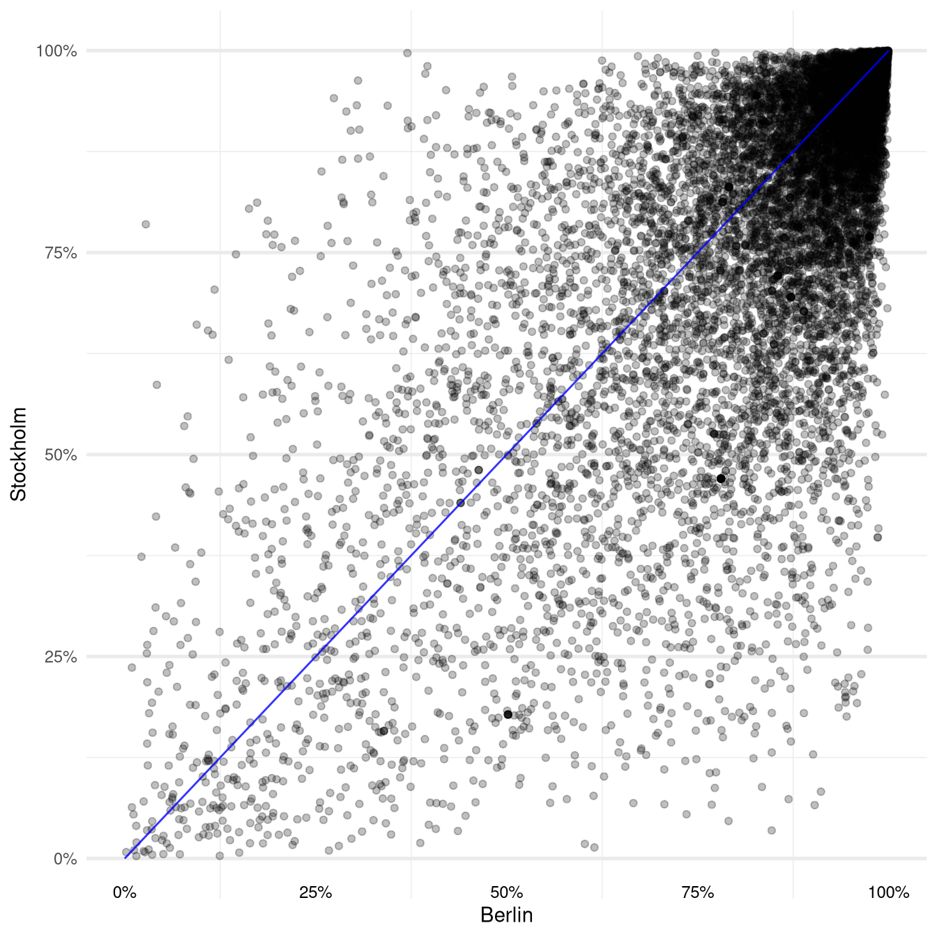
Compared to our previous model the predictions show much more variance resulting in a much more widely distributed scatter plot. This makes it slightly harder to work out if there is a pattern. But taking a closer look at the top right part of the plot one can get the impression that the average prediction difference between Berlin and Stockholm might be positive.
And indeed that is the case: on average the Berlin predictions are around 4.2 % higher than the ones from Stockholm. This puts the results of our third model between the differences we saw from our first model (6.6 %) and our second model (-0.3 %).
Conclusion
Now that we have built three different types of models, each of them producing different results, we need to ask ourselves which one of them should we trust?
The statistical aphorism “All models are wrong (but some are useful)” comes to mind and indeed choosing the “correct” model is not a trivial task.
Of the three the first one surely is the easiest to understand and interpret which is a quality that should not be underestimated, especially in an explorative setting such as ours.
However, we have identified some clear limitations of the features of that model which have raised serious doubts about the validity of some of its results.
The same criticism can be applied to the second model since it is basically using the same features. On top of that we have seen that the regularisation may play an undue role in this model, potentially hiding actually existing differences between the rating processes in the two cities.
Our third model, using the complex embeddings features certainly looks like the most powerful model and this seems to be backed up by its higher performance as measured during model validation phase. This performance however was not substantially higher than the other models and it comes at the cost of interpretability.
Finally it could be argued that each model represents another perspective on the data with neither of them being necessarily right or wrong. Therefore in the end one could even consider to combine these different perspectives in some kind of ensemble approach, taking the average of the three results as our final result (putting the difference in predictions somewhere around the 3 % mark).
In the end we could put a lot more effort into finding the right model to try and get an exhaustive and perfectly reliable answer to our initial research question. For now we will leave it at that and be content with the answers we have found and the things we have learned in the process of finding them.